5.8. Color Management

5.8.1. XYZ Color Space

Color perception, unlike spectral wavelengths, is not a directly measurable physical property. Instead, it arises from the physiological characteristics of the human visual system, making it inherently subjective.

Human vision is mediated by five types of photoreceptors. Retinal ganglion cells regulate circadian rhythms, rod cells (neuron bacilliferum) enable night vision (scotopic vision). Cone cells (neuron coniferum) are responsible for color perception and daytime vision (photopic vision). Of these, the three types of cone cells are most relevant in color management. Each type exhibits a distinct spectral sensitivity curve, which describes how it responds to different wavelengths of light. When light strikes the retina, the incident spectrum is filtered through these sensitivities to produce receptor-specific stimuli.

These three cone sensitivities are commonly referred to as L (long), M (medium), and S (short). The resulting signals define the LMS color space.

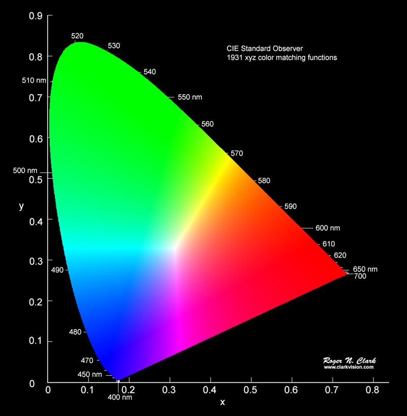
However, in practice, the XYZ color space is typically used. It is derived through a linear transformation of the L, M, and S components. The XYZ values, also known as tristimulus values, are capable of representing the entire range of colors visible to the average human observer. It is important to note that spectral sensitivity can vary slightly from person to person and may be influenced by additional factors. The figure Fig. 5.22 illustrates the standard color matching functions, which represent the average sensitivities measured from a group of observers for a 2° field of view. These measurements were conducted in 1928 and 1931 and form the basis of the CIE 1931 2° Standard Observer. These functions remain the most widely used reference for color conversion and management.

Fig. 5.22 CIE 1931 2° color matching functions

Using a spectral power distribution \(P(\lambda)\) and the three color matching functions shown in Fig. 5.22, the tristimulus values \(X\), \(Y\), and \(Z\) can be computed as follows:

(5.169)\[\begin{split}X &=\int_{\lambda} P(\lambda) \cdot x(\lambda) ~d \lambda \\ Y &=\int_{\lambda} P(\lambda) \cdot y(\lambda) ~d \lambda \\ Z &=\int_{\lambda} P(\lambda) \cdot z(\lambda) ~d \lambda\end{split}\]

Among these, the \(Y\) component corresponds to the perceived brightness of the stimulus. To convert this value into the luminous flux \(\Phi_v\), commonly used in photometry, a simple scaling by the luminous efficacy constant is applied:

(5.170)\[\Phi_v = 683 \frac{\text{lm}}{\text{W}} ~Y\]

It is important to note that the formula in (5.170) and the interpretation of \(Y\) as a luminance are only valid under conditions of photopic (daylight) vision. For mesopic (twilight) or scotopic (night) vision, different luminous efficiency functions must be used to account for the varying sensitivity of the visual system.

5.8.2. xyY Color Space

Until now, each of the three tristimulus values contained a mixture of color and brightness information. The CIE xyY color space offers a more convenient representation by separating chromaticity (color information) into the two-dimensional xy components and luminance (brightness) into the Y component. The reference point for neutral color, known as the white point, is defined by the chromaticity coordinates of the D65 standard illuminant. The spectral power distribution of D65 is designed to approximate average midday daylight in open air in Europe.

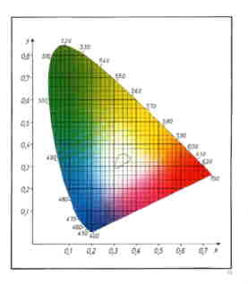
The resulting chromaticity diagram, including the D65 white point, is shown in Fig. 5.23. The spectral locus, representing monochromatic light at each visible wavelength, forms the outer boundary of the gamut, which encompasses all colors that can be represented within this system.

Fig. 5.23 xy chromaticity diagram with sRGB Gamut

XYZ to xyY

The following transformations convert CIE XYZ tristimulus values to CIE xyY color space components. These formulas are valid for \(X,~Y,~Z > 0\). If any of these values are not strictly positive, the chromaticity coordinates are set to the white point coordinates (\(x=x_r,~y=y_r\)) and \(Y\) is set to 0. The white point coordinates are typically those of the D65 standard illuminant, where \(x_r=0.31272\) and \(y_r=0.32903\) (see CIE Colorimetry, 3rd Edition, 2004, Table 11.3).

(5.171)\[\begin{split}\begin{aligned} x &= \frac{X}{X + Y + Z} \\ y &= \frac{Y}{X + Y + Z} \\ z &= \frac{Z}{X + Y + Z} = 1 - x - y\\ Y &= Y \end{aligned}\end{split}\]

Note that the \(z\) component is often omitted as its value is implicitly determined by \(x\) and \(y\) through the relationship \(x+y+z=1\).

xyY to XYZ

The inverse transformation from CIE xyY to CIE XYZ is given by:

(5.172)\[\begin{split}\begin{aligned} X &= x \cdot \frac{Y}{y} \\ Y &= Y\\ Z &= z \cdot \frac{Y}{y} \\ \end{aligned}\end{split}\]

5.8.3. sRGB Color Space

The standard RGB (sRGB) color space serves as the most common color space for digital media. Its color gamut is defined by a triangle, where any color within this triangle can be represented by a combination of its three primary colors: red, green, and blue, located at the triangle’s vertices. Given that digital monitors also typically employ three distinct light emitters per pixel, the utility of such a three-primary system becomes apparent.

sRGB utilizes the D65 white point, defined by the CIE XYZ coordinates \(X=0.95047,~Y=1,~Z=1.08883\) ([1]). It’s important to note that the sRGB gamut does not encompass the entire spectrum of visible colors, particularly lacking highly saturated colors. The sRGB gamut’s position within the broader color space is visualized in Fig. 5.23.

Color information in sRGB is typically stored with three values per pixel, each corresponding to one of the red, green, or blue channels. With a common bit depth of 8 bits per channel, the intensity range for each primary is limited to 256 discrete values. However, human perception of luminance is non-linear. Directly encoding linear intensity values within this limited range would result in a disproportionate allocation of bits, leading to fine intensity steps in some regions and coarse steps in others, potentially causing visual banding artifacts.

To mitigate this issue, sRGB values undergo a gamma correction. This non-linear transformation approximates the human eye’s luminance sensitivity, effectively distributing the available digital values more uniformly according to perceived brightness and minimizing banding.

Conversion XYZ to sRGB

The linear sRGB values, prior to gamma correction, are obtained through a linear transformation of the CIE XYZ tristimulus values. The conversion from CIE XYZ to linear sRGB is defined by the following matrix multiplication [2][3]:

(5.173)\[\begin{split}\left[\begin{array}{l} R_{\text {linear}} \\ G_{\text {linear}} \\ B_{\text {linear}} \end{array}\right]=\left[\begin{array}{ccc} +3.2404542 & -1.5371385 & -0.4985314 \\ -0.9692660 & +1.8760108 & +0.0415560 \\ +0.0556434 & -0.2040259 & +1.0572252 \end{array}\right]\left[\begin{array}{c} X_\text{D65} \\ Y_\text{D65} \\ Z_\text{D65} \end{array}\right]\end{split}\]

Applying the gamma correction results in:

(5.174)\[\begin{split}C_{\text {sRGB}}= \begin{cases}12.92\cdot C_{\text {linear}}, & C_{\text {linear}} \leq 0.0031308 \\[1.5ex] 1.055\cdot C_{\text {linear}}^{1 / 2.4}-0.055, & C_{\text {linear}}>0.0031308\end{cases}\end{split}\]

Conversion sRGB to XYZ

The inverse transformation from sRGB to XYZ is performed as follows [2][3]:

(5.175)\[\begin{split}C_{\text {linear }}= \begin{cases}\displaystyle\frac{C_{\text {sRGB}}}{12.92}, & C_{\text {sRGB}} \leq 0.04045 \\[1.5ex] \displaystyle\left(\frac{C_{\text {sRGB}}+0.55}{1.055}\right)^{2.4}, & C_{\text {sRGB}}>0.04045\end{cases}\end{split}\]

(5.176)\[\begin{split}\left[\begin{array}{l} X_{\text {D65}} \\ Y_{\text {D65}} \\ Z_{\text {D65}} \end{array}\right]=\left[\begin{array}{ccc} 0.4124564 & 0.3575761 & 0.1804375\\ 0.2126729 & 0.7151522 & 0.0721750\\ 0.0193339 & 0.1191920 & 0.9503041 \end{array}\right]\left[\begin{array}{c} R_{\text{linear}} \\ G_{\text{linear}} \\ B_{\text{linear}} \end{array}\right]\end{split}\]

Rendering Intents

As illustrated in Fig. 5.23, the sRGB color gamut does not encompass the entirety of humanly visible colors. Various approaches exist to handle colors that fall outside this gamut. The simplest is to simply clamp any negative sRGB values to zero, often resulting in inaccurate color and brightness representation. This approach is still commonly found, possibly due to its ease of implementation or a lack of awareness of better methods

[4] presents several more sophisticated gamut clipping techniques designed to minimize the visual artifacts.

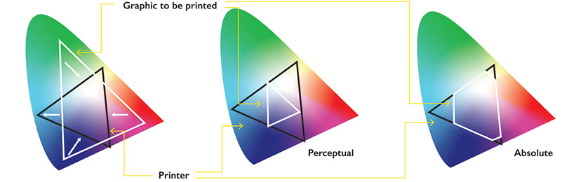
Fig. 5.24 Absolute and perceptual colorimetric rendering intent in the CIE 1976 chromaticity diagram.

Implemented Rendering Intents:

1. Ignore: This intent leaves out-of-gamut color values unmodified, delegating their handling to subsequent processing stages. Typically, this results in these values being clamped by other methods, which can introduce significant inaccuracies in hue, saturation, and brightness.

2. Absolute Colorimetric: Colors that fall within the target gamut are left unchanged. Colors outside the gamut are projected onto the gamut boundary along a straight line directed towards the white point. This method is equivalent to chroma clipping in the CIE 1931 xy chromaticity diagram.

3. Perceptual Colorimetric: This intent identifies the most saturated color that lies outside the target gamut. It then rescales the saturation of all colors in the image proportionally, such that this most saturated out-of-gamut color is brought within the gamut boundary. This technique, equivalent to chroma rescaling, is typically performed in the CIE 1976 uv chromaticity diagram, as this color space is designed such that Euclidean distances correlate well with perceived color differences.

The gamut boundary intersection for the Absolute Colorimetric mode is calculated within the CIE 1931 xy chromaticity diagram, with the projection direction determined by the white point of the D65 standard illuminant. The determination and rescaling of chroma in the Perceptual Colorimetric mode are performed in the CIE 1976 uv chromaticity diagram to better align numerical color differences with perceptual uniformity.

In its default configuration, the Perceptual Colorimetric rendering intent scales the chroma of all colors to ensure they fall within the target gamut. Alternatively, a fixed rescaling factor (within the range 0 to 1) can be supplied via the chroma_scale parameter. This allows for consistent scaling, which can be beneficial when comparing different images. In the adaptive scaling scenario, an additional L_th parameter can be specified. This parameter represents a relative luminance threshold: Colors with luminance below this threshold are excluded from the calculation of the scaling factor. This can be useful for disregarding dark but saturated image regions that might otherwise influence the overall chroma scaling. For more detailed information, refer to Color Conversions.

The effect of different rendering intents is illustrated in the next figures. The rendered images were created using the Prism. Since all spectral wavelengths create colors beyond the sRGB gamut, this leads to an extreme case. In the first image the lightness component is pictured, the following images should be the colored version of this lightness image. With the Absolute Colorimetric rendering intent one can see not only the colors having different saturation, but the lightness gradient is different compared to the first image. This can especially be seen around \(x = 1.3\) mm to \(x= 1.4\) mm. While the lightness values were in fact unchanged, this subjective difference comes from the Helmholtz-Kohlrausch effect [5], which describes that color saturation can lead to higher perceived lightness. Since the saturation was clipped, and the maximum value depends on the spectral wavelength, saturation ratios are falsified, leading to this effect behaving differently for every color. The third image shows the Perceptual Colorimetric rendering intent. One can clearly see a decreased saturation for all colors. However, the saturation ratios are kept and the lightness gradient matches the lightness image.

The effect of different rendering intents is illustrated in the following figures, generated using the Prism.This scenario represents an extreme case, due to the fact that all spectral wavelengths produce colors exceeding the sRGB gamut.

The first image depicts the lightness component. Subsequent images display the colored versions corresponding to this lightness image. Observing the result of the Absolute Colorimetric rendering intent, one can discern not only variations in color saturation but also a distinctly different lightness gradient compared to the initial image. This difference is particularly noticeable in the region between \(x = 1.3\) mm and \(x= 1.4\) mm. While the underlying lightness values remain unchanged, this subjective alteration arises from the Helmholtz-Kohlrausch effect [5], which describes how color saturation can enhance perceived lightness. As the saturation was clipped and its maximum value is dependent on the spectral wavelength, the saturation ratios are distorted, causing this effect to manifest differently for each color.

The third image demonstrates the Perceptual Colorimetric rendering intent. A clear reduction in saturation across all colors is evident. However, the chroma ratios are preserved, and the lightness gradient aligns with the original lightness image.

Table 5.5 Difference in different sRGB rendering intents.

A lot of negative examples for color representation can be found in literature (Link1, Link2, Link3, Link4).

In most cases, negative sRGB values were simply clipped, leading to distortions not only in saturation but also in hue and brightness. For example, colors near 510 nm are rendered as deep green instead of a more nuanced greenish-cyan. In some instances, even representable colors within the gamut are inaccurate, which can be observed as overly saturated colors throughout the diagram.

Conversely, positive examples can be found at: Link6 Link7

It is important to note that these positive examples utilize a different luminance normalization, displaying the colors with increased brightness.

5.8.4. CIELUV Color Space

A limitation of the XYZ color space lies in the interdependence of color and brightness. Furthermore, the perceived distances in brightness and color are not linear within this space. To address these issues, the improved CIE 1976 L, u, v color space (abbreviated as CIELUV) was developed.

In CIELUV, L represents the lightness component, while u corresponds to the red-green axis and v to the blue-yellow axis. The white point can be freely chosen, although the D65 standard illuminant is commonly used.

Analogous to the XYZ color space, a chromaticity diagram can be derived, with coordinates denoted as \(u',~v'\). This diagram is also known as the CIE 1976 UCS (uniform chromaticity scale) diagram and is illustrated in Figure Fig. 5.25. As its name implies, the UCS diagram exhibits uniform geometric distances throughout, where equal distances correspond to equal perceived color differences. This uniformity is not present in the CIE 1931 chromaticity diagram shown in Figure Fig. 5.23. Consequently, the UCS diagram is the appropriate tool for visualizing the extent of the color ranges absent in the sRGB gamut.

Fig. 5.25 u’v’ chromaticity diagram with sRGB Gamut

Another widely adopted CIE model is the CIELAB color space, which employs the same lightness function as CIELUV but utilizes different color components. For color mixing and additive color applications, CIELUV is generally preferred due to its associated chromaticity diagram (as previously mentioned) and a defined mathematical expression for color saturation [6].

XYZ to CIELUV

Conversion formulas are based on [7]. These equations are valid for \(X, Y, Z > 0\). Otherwise, we define \(L = 0, ~u=0,~v=0\).

(5.177)\[\begin{split}\begin{aligned} &L= \begin{cases}116 \sqrt[3]{y_r}-16 & \text { if } y_r>\epsilon \\ \kappa y_r & \text { otherwise }\end{cases} \\ &u=13 L\left(u^{\prime}-u_r^{\prime}\right) \\ &v=13 L\left(v^{\prime}-v_r^{\prime}\right) \end{aligned}\end{split}\]

With the following parameters:

(5.178)\[\begin{split}\begin{aligned} \epsilon &= 0.008856\\ \kappa &= 903.3\\ y_r &=\frac{Y}{Y_r} \\ u^{\prime} &=\frac{4 X}{X+15 Y+3 Z} \\ v^{\prime} &=\frac{9 Y}{X+15 Y+3 Z} \end{aligned}\end{split}\]

Here, \(Y_r\) is derived from the white point coordinates \((X_r,~Y_r,~Z_r)\), typically those of the standard illuminant D65. Conversely, \(u'_r\) and \(v'_r\) represent the \(u', ~v'\) values calculated for these white point coordinates.

CIELUV to XYZ

Conversion formulas are based on [8]. Note that some formulas have been reformulated for clarity. These equations are valid for \(L > 0\). If \(L = 0\), then all values are set to \(X=Y=Z=0\).

(5.179)\[\begin{split}Y= \begin{cases}\left(\frac{L+16} {116}\right)^3 & \text { if } L>\kappa \epsilon \\ L / \kappa & \text { otherwise }\end{cases}\end{split}\]

(5.180)\[\begin{split}\begin{aligned} X &= \frac{9}{4} \cdot \frac{u + 13 L u'_r}{v + 13 L v'_r}\\ Z &= 3 Y \cdot \left(\frac{13 L}{v + 13 L v'_r} - \frac{5}{3}\right) - \frac{X}{3}\\ \end{aligned}\end{split}\]

CIELUV to u’v’L

For \(L > 0\), the following equations apply. If \(L = 0\), we set \(u' = u'_r, ~v' = v'_r\).

(5.181)\[\begin{split}\begin{aligned} L &= L\\ u' &= u'_r + \frac{u}{13 L}\\ v' &= v'_r + \frac{v}{13 L}\\ \end{aligned}\end{split}\]

CIELUV Chroma

Chroma calculation based on [9]:

(5.182)\[C = \sqrt{u^2 + v^2}\]

CIELUV Hue

Hue calculation based on [9]:

(5.183)\[H = \text{arctan2}(v, u)\]

CIELUV Saturation

Saturation calculation based on [10]: These equations are valid for \(L > 0\). If \(L = 0\), we set \(S=0\).

(5.184)\[S = \frac{C}{L}\]

5.8.5. sRGB Spectral Upsampling

While the conversion of a physical light spectrum to coordinates within a human vision color model is a frequent task, the reverse process is less common. In our application, this inverse conversion is employed to load digital images into the raytracer and propagate spectral wavelengths throughout the tracing geometry. Such an implementation facilitates straightforward simulations of diverse light and lighting scenarios.

This conversion process is commonly known as Spectral Upsampling, Spectral Rendering, or Spectral Synthesis. An implementation utilizing real LED spectral curves can be found in [11], while methods for modeling sRGB reflectances are detailed in [12] and [13].

It is crucial to recognize that not all chromaticities within human vision, and even the sRGB gamut, can be accurately modeled by valid reflectance spectra, as the reflectance range is constrained to \([0,~1]\). However, this limitation does not apply when selecting illuminant curves.

While the conversion of a spectral distribution to a color is well-defined, going backwards the conversion is not unique and simply reversible. Multiple spectral distributions can create the same color stimulus, an effect known as metamerism. In fact, there infinitely many distributions being perceived as the same color. With so many possibilities to choose from, we can demand some requirements for our sRGB primaries:

While the conversion from a spectral distribution to a color is a well-defined process, the reverse conversion is neither unique nor simply reversible. Multiple distinct spectral distributions can evoke the same color perception, a phenomenon known as metamerism. In fact, an infinite number of spectral distributions can be perceived as identical colors. Given this vast number of possibilities, we can establish certain requirements for our sRGB primaries:

Requirements

1. Same color coordinates as the sRGB primaries

2. Same luminance ratios as sRGB primaries

3. Simple, smooth spectral functions

4. Wide spectrum

5. Relatively few light in non-visible regions (infrared and ultraviolet)

Points 1 and 2 simplify the spectral upsampling process because the mixing ratios of the linear sRGB values can be directly utilized. Although we could theoretically define a new color space and gamut that encompasses the sRGB gamut but is significantly broader, this approach would necessitate additional color space conversions. Furthermore, it would result in narrower spectra, which contradicts point 4. It is essential to use linear sRGB values, as they are proportional to the physical intensity of the sRGB primaries. In contrast, standard sRGB values are gamma-corrected to approximate the non-linear response of human vision.

Points 3 and 4 are necessary to approximate natural illuminants with a high degree of realism. Superimposing all sRGB primaries to generate a white spectrum should ideally cover the entire visible spectral range without any significant gaps. Such gaps would reduce the color rendering index (CRI) of the illuminant. The CRI is a metric used to quantify how faithfully an object’s colors are rendered when illuminated by a particular light source. For example, a light spectrum with a deficiency in the yellow region would fail to accurately render pure yellow colors.

Point 5 ensures that the majority of the traced light contributes meaningfully to the final rendered image. Given that sRGB is a color space designed for human vision, an input color image in sRGB should ideally produce a rendered image with colors perceived by humans. Tracing rays with colors far outside the visible spectrum would constitute an inefficient use of rendering time.

In theory, we could derive spectra for the sRGB primaries by combining a D65 white spectrum with the reflectance curves described in the previously cited works. However, this approach has drawbacks: the resulting spectra would lack smoothness due to the non-smooth nature of the D65 spectrum, and a significant portion of the spectrum would fall within the range of human invisibility or near-invisibility. Furthermore, there are no straightforward mathematical descriptions for the resulting spectral curves.

Table 5.6 sRGB primary specification, see [14]

Color value	Red	Green	Blue	D65
\(x\)	0.6400	0.3000	0.1500	0.3127
\(y\)	0.3300	0.6000	0.0600	0.3290
\(z\)	0.0300	0.0100	0.7900	0.3583
\(Y\)	0.2127	0.7152	0.0722	1.0000
sRGB	[1, 0, 0]	[0, 1, 0]	[0, 0, 1]	[1, 1, 1]

Dimensioning

The mathematical functions of choice is a Gaussian function, which is defined as:

(5.185)\[S(\lambda, \mu, \sigma)=\frac{1}{\sqrt{2 \pi \sigma^{2}}} \exp \left(-\frac{(\lambda-\mu)^{2}}{2 \sigma^{2}}\right)\]

A Gaussian function presents itself as a suitable choice due to its smooth, bell-shaped curve and its widespread application across various fields. Moreover, the principle of maximum entropy [15] advocates for this type of function when dealing with the two parameters of position and width, as it represents the probability distribution that maximizes uncertainty for a given set of constraints.

Employing optimization methods in Python, the following Gaussian functions were derived, exhibiting the same color stimulus as the sRGB primaries:

(5.186)\[\begin{split}r_0(\lambda) =&~ 75.1660756583 \cdot \Big[ S(\lambda, 639.854491, 30.0)\\ & + 0.0500907584 \cdot S(\lambda, 418.905848, 80.6220465)\Big]\\ g_0(\lambda) =&~ 83.4999222966 \cdot S(\lambda, 539.13108974, 33.31164968)\\ b_0(\lambda) =&~ 47.99521746361 \cdot \Big[ S(\lambda, 454.833119, 20.1460206)\\ & + 0.184484176 \cdot S(\lambda, 459.658190, 71.0927568)\Big]\\\end{split}\]

The spectral distribution of the green primary is modeled using a single Gaussian function, whereas the red and blue primaries utilize a superposition of two Gaussian functions each. This choice is informed by Figure 3a in [16], which demonstrates that the chromaticity coordinates of the red primary cannot be accurately reproduced with a single Gaussian curve. While it is theoretically possible to represent the blue primary’s chromaticity with a single Gaussian, this would only be feasible for narrow illuminants characterized by a small standard deviation. To allow for greater flexibility in selecting the spectrum width, two Gaussian functions are also employed for the blue primary.

It is important to note that the initial luminance ratios of these Gaussian approximations differ from those of the standard sRGB primaries. To address this discrepancy, we need to rescale the functions to match the correct luminance ratios. The scaling factor for the green curve is maintained at a value of 1, and the rescaling factors for the red and blue curves are determined as follows:

(5.187)\[\begin{split}r(\lambda) =&~ 0.951190393 \cdot r_0(\lambda)\\ g(\lambda) =&~ 1.000000000 \cdot g_0(\lambda)\\ b(\lambda) =&~ 1.163645855 \cdot b_0(\lambda)\\\end{split}\]

The resulting spectrum for sRGB white (with coordinates \([1.0, 1.0, 1.0]\)) is illustrated in Fig. 5.26.

Fig. 5.26 Simulated sRGB white spectrum.

Note

The Gaussian curves additionally include a cutoff at \(\lambda = 380\,\) nm and \(\lambda = 780\,\) nm. This ensures that all derived ratios and constants remain consistent, even if the simulated wavelength range is extended beyond these default boundaries.

In a subsequent step, the spectral distributions of the color channel primaries are treated as probability density functions (pdfs). A key property of a pdf is that its integral over the entire domain (the area under the curve) must be normalized to unity, representing a total probability of 1. This normalization process effectively cancels out any multiplicative factors in the channel curves, as well as the relative scaling between the channels. To compensate for this effect on luminance, the mixing ratio of each channel is rescaled by the area under its corresponding spectral curve. Since this area is proportional to the probability ratio, this rescaling effectively transfers the information about channel luminance from the absolute magnitudes of the curve values to the relative probabilities of the channels.

The area scaling factors are:

(5.188)\[\begin{split}r_\text{P} = 0.885651229244\\ g_\text{P} = 1.000000000000\\ b_\text{P} = 0.775993481741\\\end{split}\]

As the calculated rescaling factors indicate, the red and blue channels have smaller factors compared to the green channel. This is visually apparent in the preceding figure, where the areas under the red and blue primary curves are smaller than that under the green primary curve.

Following the selection of a color channel based on the linear sRGB mixing ratios (which have been scaled by the aforementioned factors), the corresponding channel primary spectral curve is then treated as a probability density function. A specific wavelength is subsequently sampled from this probability distribution.

Example

Choose random wavelengths from sRGB value \(\text{RGB} = [1.0, 0.5, 0.2]\).

1. Convert to linear sRGB: \([1.000, 0.214, 0.033]\)

2. Rescale by area/probability factors \(r_\text{P}, g_\text{p}, b_\text{p}\): We get approximately \([0.886, 0.214, 0.025]\)

3. Normalize, so integral equals 1: \([0.788, 0.190, 0.022]\)

4. Choose one of the three channels with the values from 3. as the probability: The R channel gets randomly chosen.

5. Use the R primary curve as probability distribution, choose a random wavelength accordingly: \(\lambda = 623.91\,\) nm gets chosen.

6. Repeating 4. and 5. by choosing randomly, a spectrum is created, that for many rays converges to the correct sRGB color.

Brightness Sampling

While the previously described procedure ensures accurate color representation, it is also crucial to account for the brightness of each pixel in the image. To correctly represent the pixel intensity, each pixel is assigned a probability proportional to its intensity.

This pixel intensity is calculated by first converting the sRGB color values to linear sRGB and then multiplying each linear channel value by its corresponding overall power, which is proportional to \(r_\text{P}, g_\text{P}, b_\text{P}\). These scaled channel values are then summed together to obtain the pixel intensity.

Subsequently, each pixel is assigned an intensity weight based on this calculated intensity. To ensure proper probabilistic sampling across the entire image, these intensity weights are then rescaled so that the sum over all pixels in the image equals 1.

Example

Choose random pixels from the image below

(5.189)\[\begin{split}\text{Image} = \begin{bmatrix} [1.0, 0.0, 0.2] & [0.0, 0.0, 0.0]\\ [0.1, 0.5, 1.0] & [1.0, 0.2, 1.0] \end{bmatrix}\end{split}\]

1. Convert to linear sRGB

(5.190)\[\begin{split}\begin{bmatrix} [1.000, 0.000, 0.033] & [0.000, 0.000, 0.000]\\ [0.010, 0.214, 1.000] & [1.000, 0.033, 1.000] \end{bmatrix}\end{split}\]

2. Multiply by area factors \(r_\text{P}, g_\text{P}, b_\text{P}\) and sum all channels for each pixel

(5.191)\[\begin{split}\begin{bmatrix} 0.911 & 0.000\\ 0.999 & 1.694 \end{bmatrix}\end{split}\]

3. Normalize weights

(5.192)\[\begin{split}\begin{bmatrix} 0.253 & 0.000\\ 0.277 & 0.470 \end{bmatrix}\end{split}\]

4. Chose randomly according to the probabilities.

---

References

[1]

Wikipedia. Illuminant D65. 2022. URL: https://en.wikipedia.org/wiki/Illuminant_D65 (visited on 2022-12-01).

[2] (1,2)

Bruce Lindbloom. RGB/XYZ Matrices. 2017. URL: http://brucelindbloom.com/index.html?Eqn_RGB_XYZ_Matrix.html (visited on 2022-12-01).

[3] (1,2)

Wikipedia. sRGB. 2022. URL: https://de.wikipedia.org/wiki/SRGB (visited on 2022-12-01).

[4]

Björn Ottosson. sRGB gamut clipping. 2021. URL: https://bottosson.github.io/posts/gamutclipping/ (visited on 2022-12-12).

[5] (1,2)

Wikipedia. Helmholtz–Kohlrausch effect. 2022. URL: https://en.wikipedia.org/wiki/Helmholtz%E2%80%93Kohlrausch_effect (visited on 2022-12-01).

[6]

Adrian Ford and Alan Roberts. Colour space conversions. 1998. URL: https://poynton.ca/PDFs/coloureq.pdf (visited on 2024-09-04).

[7]

Bruce Lindbloom. XYZ to Luv. 2017. URL: http://www.brucelindbloom.com/index.html?Eqn_XYZ_to_Luv.html (visited on 2022-12-01).

[8]

Bruce Lindbloom. Luv to XYZ. 2017. URL: http://www.brucelindbloom.com/index.html?Eqn_Luv_to_XYZ.html (visited on 2022-12-01).

[9] (1,2)

Jim Schwiegerling. Field Guide to Visual and Ophthalmic Optics. SPIE, 2004. URL: https://doi.org/10.1117/3.592975, doi:10.1117/3.592975.

[10]

Wikipedia. Colorfulness. 2022. URL: https://en.wikipedia.org/wiki/Colorfulness (visited on 2022-12-01).

[11]

Giuseppe Claudio Guarnera, Yuliya Gitlina, Valentin Deschaintre, and Abhijeet Ghosh. Spectral Upsampling Approaches for RGB Illumination. In Abhijeet Ghosh and Li-Yi Wei, editors, Eurographics Symposium on Rendering. The Eurographics Association, 2022. doi:10.2312/sr.20221150.

[12]

Ian Mallett and Cem Yuksel. Spectral Primary Decomposition for Rendering with sRGB Reflectance. In Tamy Boubekeur and Pradeep Sen, editors, Eurographics Symposium on Rendering - DL-only and Industry Track. The Eurographics Association, 2019. doi:10.2312/sr.20191216.

[13]

Scott A. Burns. Fast rgb to spectrum conversion for reflectances. http://scottburns.us/fast-rgb-to-spectrum-conversion-for-reflectances/, 2018. Accessed: 2024-11-20.

[14]

Wikipedia. sRGB. 2022. URL: https://en.wikipedia.org/wiki/SRGB (visited on 2022-12-01).

[15]

Wikipedia. Maximum entropy probability distribution. 2024. URL: https://en.wikipedia.org/wiki/Maximum_entropy_probability_distribution (visited on 2024-11-21).

[16]

Roger N. Clark. Color Part 1: - CIE Chromaticity and Perception. 2020. URL: https://clarkvision.com/articles/color-cie-chromaticity-and-perception/ (visited on 2022-12-12).