4.9. Focus Search

4.9.1. Focus Modes

Focus search is available with these four methods:

"RMS Spot Size"	minimal variance of the lateral ray position
"Irradiance Variance"	highest irradiance variance
"Image Sharpness"	sharpest edges of the full image
"Image Center Sharpness"	sharpest edges in the center region of the image

These methods utilize all available rays, so tracing the scene with a larger number of rays is favorable. Detailed descriptions of these methods are found below. Focus search methods should be chosen according to the simulation and geometry scenario:

Case 1: Perfect, nearly ideal focal point

• Examples: Focus of an ideal lens. Paraxial illumination of a real lens.

• Preferred methods: RMS Spot Size. Irradiance Variance is also suitable, but has worse performance.

In the below example, both RMS Spot Size and Irradiance Variance find a similar focal position, differing only in 70 µm. Note the different scaling of the images.

Table 4.12 Comparison between “RMS Spot Size” (left) and “Irradiance Variance” (right) in linear (top) and logarithmic lightness values (bottom). Example file: Double Gauss. Focus search on ray source 0 only. 2 million rays.

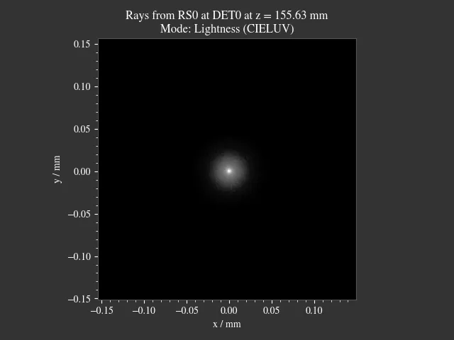
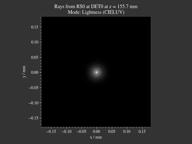
Case 2: Strong aberrations or no distinct focal point

• Examples: Lens with large amounts of spherical aberration, multifocal lens

• Preferred methods: Irradiance Variance.

The following example showcases a setup with noticeable amounts of spherical aberration. The method RMS Spot Size tries the minimize the radial distance of the outer rays, while also sacrificing a sharp core. Irradiance Variance correctly finds a suitable focal position. In the logarithmic plots below, the outer rays are more discernible. While they merely contribute in the right image, they severely raise the RMS-value, preventing the RMS to choose this actually superior solution.

Table 4.13 Comparison between “RMS Spot Size” (left) and “Irradiance Variance” (right) in linear (top) and logarithmic lightness values (bottom). Rendered in the example geometry Spherical Aberration.

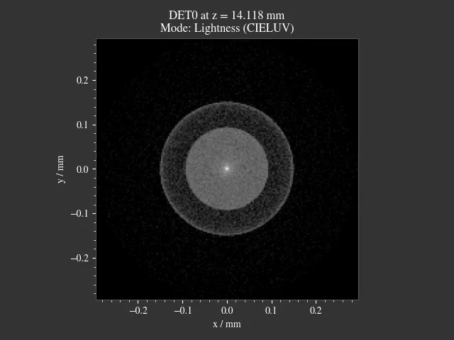
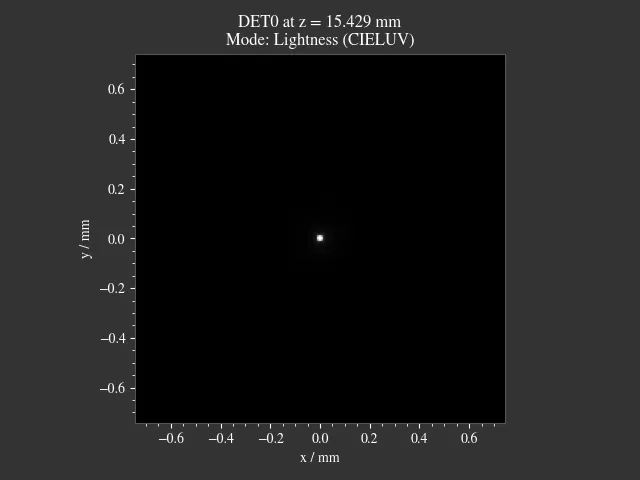
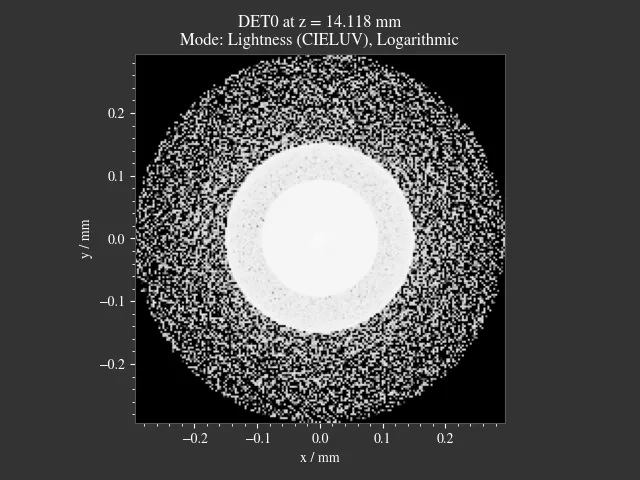
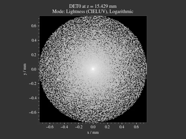
Case 3: Finding the optimal image distance

• Example: Actual best image position (not just the paraxial) in a multi-lens setup.

• Preferred methods: Image Sharpness. With large amounts of curvature of field Image Center Sharpness should be selected instead, to find a best-fit focus for the center region.

For best results, a target with high contrast and sharp edges should be set as source image. Examples include the Siemens star or the grid preset, the latter is depicted in table Table 4.8.

The following two figures demonstrate the Image Sharpness focussing for a setup with distinct field of curvature. While the left part shows a best-focus fit for the whole image, the right part was optimized for the image center.

Table 4.14 Comparison between “Image Sharpness” (left) and “Image Center Sharpness” (right) for a setup with large amounts of field of curvature. Example Image Render with a grid image selected, a pupil of 1mm and 5 million rays simulated.

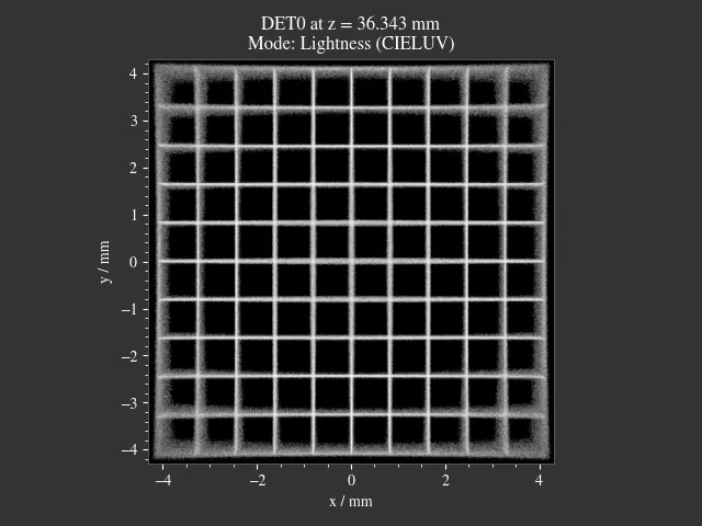
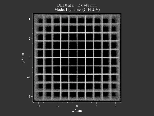
4.9.2. Limitations

Limitations of the focus search include:

• due to restrictions on the search region, foci inside a surface (between minimum and maximum z-value of a surface) can’t be found

• absorptions at the raytracer outline are not handled, when they occur inside the search region. This region reaches from the last to next surface in z-direction

• in more complex cases, only a local minimum is found, but not the global one

• see the limitations of each method below

4.9.3. Usage

The focus_search method takes the focus mode and a starting position as parameters. With this starting position, the search region is defined as axial maximum z-position of the last surface in negative z-direction to the axial minimum of the next position in z-direction. This includes surfaces from ray sources, lenses, filters, apertures as well as the outline planes. Before focus search, the Raytracer geometry needs to be traced first.

res, fsdict = RT.focus_search("RMS Spot Size", 12.09)

This function returns a two-element tuple, where the first one is a scipy.optimize.OptimizeResult with information on the root finding. The found z-position is accessed with res.x. The second return value includes some additional information required for the Focus Search Cost Function Plots.

By default, the focus search includes rays from all sources. Optionally a source_index parameter can be provided to limit the search to a specific ray source.

res, fsdict = RT.focus_search("RMS Spot Size", 12.09, source_index=1)

If the output dictionary fsdict should include sampled cost function values, the parameter return_cost must be set to True:

res, fsdict = RT.focus_search("RMS Spot Size", 12.09, return_cost=True)

This is required for plotting the cost function using focus_search_cost_plot, see Focus Search Cost Function Plots. It is deactivated by default to increase the performance of methods "RMS Spot Size", "Irradiance Variance"

4.9.4. Cost Function Plot

Checking if the optimization found a suitable optimum is done with Focus Search Cost Function Plots.

4.9.5. Cost Function Details

4.9.5.1. RMS Spot Size

This function minimizes the position variance \(\sigma^2\) of lateral ray positions \(x\) and \(y\) at axial position \(z\). All positions are weighted according to their power \(P\) when calculating the weighted variance \(\sigma^2_P\). The Pythagorean sum is applied for a simple quantity \(R_\text{v}\) for optimization.

(4.22)\[\underset{z \in [z_0, z_1]}{\text{minimize}}~~ R_\text{v}(z) := \sqrt{\sigma^2_{x,P}(z) + \sigma^2_{y,P}(z)}\]

This procedure is simple to implement and performant. However, minimizing the overall position variance is disadvantageous in many cases: For example, for an outlying halo, the method also tries to minimize the spread of these outer rays, which leads to a compromise between the halo and actual focus size.

4.9.5.2. Irradiance Variance

The mode Irradiance Variance renders a two dimensional power histogram \(P(x, y, z)\) for rays at position \(z\). Dividing each pixel by its area generates an irradiance image \(E(x, y, z)\). This method then calculates the variance of these values and locates the position \(z\) with the largest variance.

(4.23)\[\underset{z \in [z_0, z_1]}{\text{maximize}}~~ \log{\sigma_E^2(z)}\]

Applying the logarithm leads to a more compact and stable value range of the cost function.

The variance increase for low entropy images (= defined details) and for images with high irradiance (= power/area).

The image dimensions are defined by the outermost rays, the absolute image size therefore varies along the beam path. This can lead to issues with marginal rays far from the optical axis, as these rays increase the pixel size for a specified fixed pixel count.

4.9.5.3. Image Sharpness

For this method, a power histogram is calculated in the same manner, but the pixel values are not normalized by their area. The method then maximizes all image gradients, which indicate sharp structures and a high local variance. The magnitude of the gradient is calculated from the Pythagorean sum of its components. Maximizing the sum of all squared magnitudes leads to the following expression:

(4.24)\[\underset{z \in [z_0, z_1]}{\text{maximize}} ~~ \sum_{x, y} \left(\left( \frac{\partial P(x, y, z)}{\partial x}\right)^2 + \left( \frac{\partial P(x, y, z)}{\partial y}\right)^2\right)\]

This is equivalent to:

(4.25)\[\underset{z \in [z_0, z_1]}{\text{maximize}}~~ \sum_{x,y} \left( \frac{\partial P(x, y, z)}{\partial x}\right)^2 + \sum_{x, y} \left( \frac{\partial P(x, y, z)}{\partial y}\right)^2\]

4.9.5.4. Image Center Sharpness

Compared to the Image Sharpness method, the image is weighted with a rotationally symmetric Hanning window:

(4.26)\[\begin{split}P_w(x, y, z) = P(x, y, z) \cdot \begin{cases} 1 + \cos(\pi r) &~~\text{for}~ r \leq 1\\ 0 & ~~\text{for}~ r > 1\\ \end{cases}\end{split}\]

Here, \(r\) is calculated from the normalized image coordinates \(x, y \in [-1, 1]\). As moving gradients towards regions with higher weights also increases \(P_w\), the windowed image power is normalized first to avoid rewarding images with more central image components.