3. Quickstart
The library comes with a variety of different example scripts that are described in Section 1. You can download the full examples.zip archive here.
The spherical_aberration.py script provides a good quickstart introduction. Below you can find its code with detailed comments.
Content of examples/spherical_aberration.py:
1#!/usr/bin/env python3
2# ^-- shebang for simple execution on Unix systems
3
4# This quickstart example demonstrates some features of optrace.
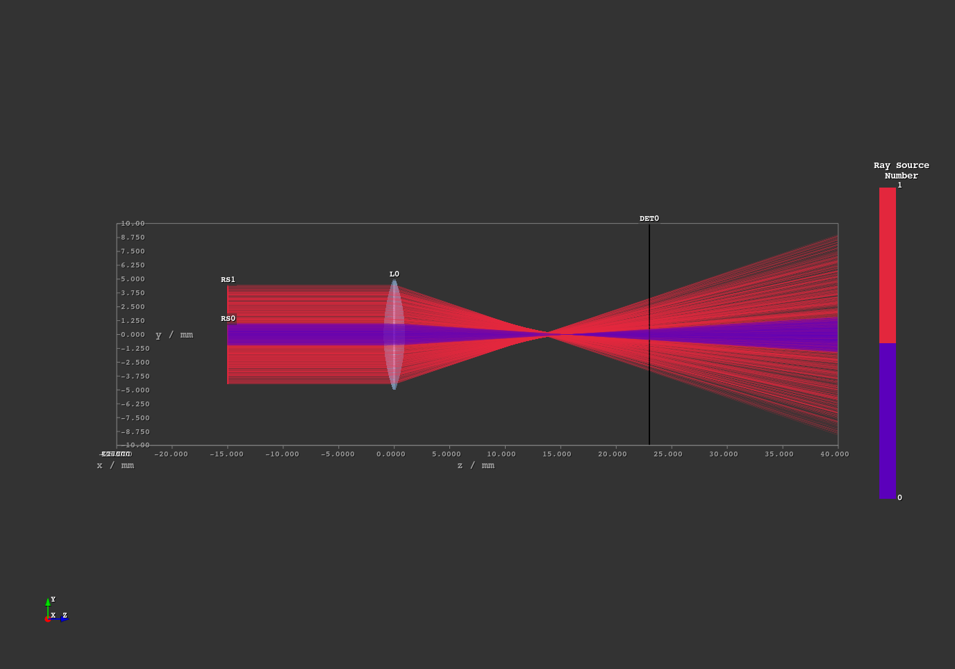
5# The goal is to investigate the spherical aberration of a simple lens.
6
7# Make sure the optrace library is installed on your system.
8
9# First, we need to import the optrace package and its GUI.
10# GUI and raytracer are separated, so we don't have the overhead of always loading all external libraries.
11import optrace as ot
12from optrace.gui import TraceGUI
13
14# A Raytracer object provides the raytracing functionality and also controls the tracing geometry.
15# The outline parameter specifies a three dimensional box, in which the geometry and all rays are located.
16# The values are specified as [x0, x1, y0, y1, z0, z1], with x1 > x0, y1 > y0 and z1 > z0.
17# All coordinates in the tracing geometry are specified in millimeters.
18RT = ot.Raytracer(outline=[-10, 10, -10, 10, -25, 40])
19
20# All elements in the geometry (sources, lenses, detectors, ...) consist of Surfaces.
21# A Surface describes a specific height behavior (z) depending on 2D x,y-coordinates relative to the surface center.
22# For the RaySource we define a circular surface with radius 1mm, which is perpendicular to the z-axis.
23# Its absolute position in the scene is controlled by the parent object.
24RSS0 = ot.CircularSurface(r=1)
25
26# A RaySource generates the rays for raytracing. It consists of an emitting surface, a ray divergence behavior,
27# a specific light spectrum, a specific base orientation of the rays as well as a specific polarization.
28# Parallel light (divergence="None") parallel to the z-axis is specified by a orientation vector of s=[0, 0, 1].
29# The light spectrum is chosen as daylight spectrum D65, which can be found in the presets submodule.
30RS0 = ot.RaySource(RSS0, divergence="None", spectrum=ot.presets.light_spectrum.d65,
31 pos=[0, 0, -15], s=[0, 0, 1])
32# After its creation the element needs to be added to the tracing geometry.
33RT.add(RS0)
34
35# Next, we create a RaySource with a RingSurface.
36# A ring is parametrized by an additional inner circle with radius ri.
37RSS1 = ot.RingSurface(r=4.5, ri=1)
38RS1 = ot.RaySource(RSS1, divergence="None", spectrum=ot.presets.light_spectrum.d65, pos=[0, 0, -15], s=[0, 0, 1])
39RT.add(RS1)
40
41# Next, we define a Lens with a constant refraction index of 1.5.
42# The index is specified as RefractionIndex object with mode "Constant" and a value of n=1.5.
43# Besides constant values, RefractionIndex supports different wavelength-dependent models and even custom behavior.
44n = ot.RefractionIndex("Constant", n=1.5)
45
46# A lens consists of a front and back surface.
47# In the case of spherical lens surfaces, we need to specify a surface radius r and a curvature radius R.
48# For a biconvex lens the front has a positive curvature and the back a negative one.
49front = ot.SphericalSurface(r=5, R=15)
50back = ot.SphericalSurface(r=5, R=-15)
51# The creation of the lens requires both surfaces, as well as a position and a refractive index.
52# There are multiple ways to define the overall lens thickness:
53# In our case we provide the parameter de, which is a thickness extension between front and back surface.
54# This means that there is a spacing of de=0.2mm between the end of the front surface and the start of the back surface.
55# The Lens position parameter pos then defines the geometric center of these 0.2mm.
56L = ot.Lens(front, back, de=0.2, pos=[0, 0, 0], n=n)
57RT.add(L)
58
59# A Detector renders images inside the Raytracer scene and is geometrically defined by a single surface.
60# For a rectangular detector with side lengths of 20mm a RectangularSurface with a "dim" of [20, 20] is defined:
61DETS = ot.RectangularSurface(dim=[20, 20])
62# A detector takes a Surface and a position as arguments
63DET = ot.Detector(DETS, pos=[0, 0, 23.])
64RT.add(DET)
65
66# After the geometry definition, the optical setup must be simulated next.
67# This could be done by either calling RT.trace(N), with N being the number of rays,
68# or by creating a graphical frontend, that automatically traces the scene.
69
70# Such a TraceGUI object requires the raytracer as parameter and supports different visualization setting parameters.
71# For example, rays will be colored according to their source number by providing color_type="Source",
72# while a higher relative ray opacity is set by ray_opacity=0.2.
73sim = TraceGUI(RT, coloring_mode="Source", ray_opacity=0.2)
74
75# The GUI is started by calling run().
76sim.run()
77
78# You can now experiment with different features:
79# 1. Navigate in the three dimensional geometry scene.
80# 2. Click on ray-surface intersections to display different ray properties.
81# 3. Play around with visual settings in the main tab.
82# 4. Move the detector and render detector images in the Imaging-Tab.
83# 5. Do a Focus search for each of the two sources.
84# In the "Focus" Tab select "Rays From Selected Source Only" and click on the "Find Focus" Button.
85# Select the other ray source to find the second focus.
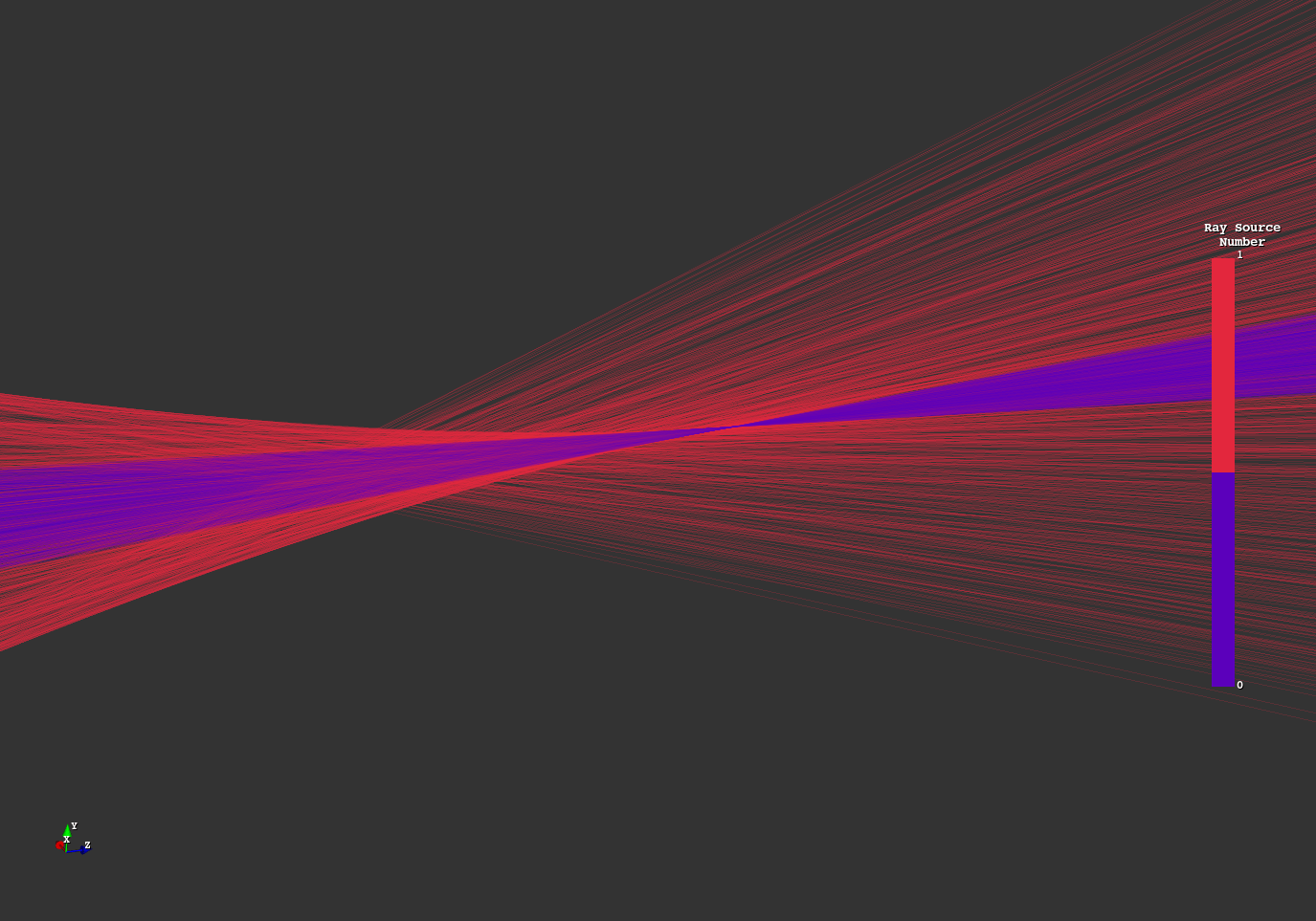
86
Screenshots