4.5. Raytracer
4.5.1. Raytracer
Overview
The Raytracer class provides the functionality for tracing, geometry checks, focus search,
and rendering spectra and images.
Since the Raytracer is a subclass of a Group,
elements can be changed or added in the same way as described in Section 4.4.1.
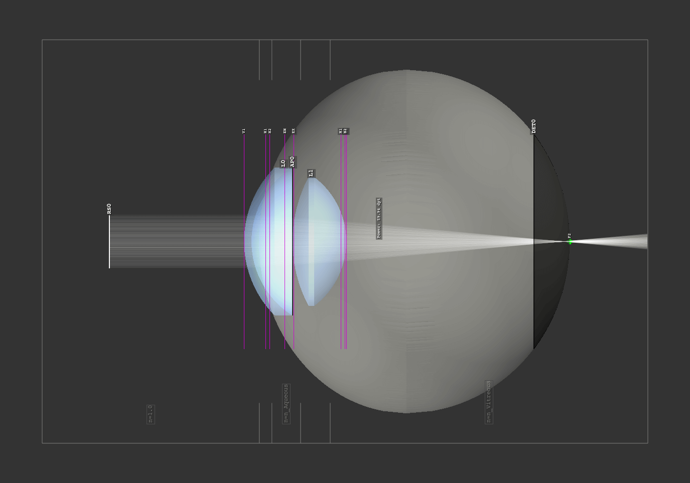
Fig. 4.19 Example of a raytracer geometry as side view in the TraceGUI.
Outline
All objects and rays only exist in a three-dimensional box, the outline.
It is a required parameter when initializing the Raytracer:
RT = ot.Raytracer(outline=[-2, 2, -3, 3, -5, 60])
The outline is provided as six element list with positions \([x_0, x_1, y_0, y_1, z_0, z_1]\)
defining the outer boundaries.
Geometry
As optrace implements sequential raytracing, all surfaces and objects must be in a well-defined
and unique chronological sequence along the optical axis.
This applies to all elements with interactions of light (Lens, IdealLens, Filter, Aperture, RaySource).
The elements Detector, LineMarker, PointMarker, BoxVolume, SphereVolume, CylinderVolume
are excluded from this. All ray source elements must lie prior to any lenses, filters and apertures.
All subsequent lenses, filters, and apertures must not collide with each other and must be inside the outline.
Rays hitting the outline box are absorbed in any case.
Surrounding Media
In Section 4.3.3 we learned that when creating a lens, the n2 parameter defines the subsequent medium.
In the case of multiple lenses, the n2 of the previous lens is the medium prior to the next lens.
For the raytracer, we can define an n0 which defines the refractive index for all
unspecified n2 media, as well as for the region in front of the first lens.
The following figure shows a setup with lenses L0, L2 having a n2 defined and a custom
n0 parameter in the raytracer class. The medium before the first lens as well as the medium
behind L1 are therefore set to n0.

Fig. 4.20 Schematic figure of a setup with a ray source, three different lenses and three different ambient media
Absorbing Rays
optrace ensures that rays not intersecting both lens surfaces are absorbed.
Generally, these rays are seen as error cases. A ray only hitting one surfaces must enter/leave through the lens side cylinder, that is not handled in our sequential simulation. Rays not hitting the lens at all are typically undesired. In real optical systems they would be absorbed by the housing of the system.
Parameter no_pol
The raytracer provides the functionality to trace polarization directions. Doing so, not only the polarization vector for the ray and ray segment is calculated, but also the exact transmission at each surface transition. Unfortunately, these calculations are comparatively computationally intensive.
With the parameter no_pol=True no polarizations are calculated and an unpolarized/uniformly polarized light
is assumed everywhere. Typically this speeds up the tracing by 10-30%.
Whether the influence of polarization can be neglected depends on the exact optical setup and application.
4.5.2. Tracing
Tracing the system
Run the tracing with the Raytracer.trace()
method of the Raytracer class.
It takes the number of rays N as parameter.
The method uses the current tracing geometry and stores the ray properties
internally in a RayStorage object.
Example
Below you can find an example. An eye preset is loaded and flipped around the x-axis. A point source is added near the retina and the geometry is traced.
import optrace as ot

# init raytracer
RT = ot.Raytracer(outline=[-10, 10, -10, 10, -10, 60])

# load eye preset
eye = ot.presets.geometry.arizona_eye(pupil=3)

# flip, move and add it to the tracer
eye.flip()
eye.move_to([0, 0, 0])
RT.add(eye)

# create and add divergent point source
point = ot.Point()
RS = ot.RaySource(point, spectrum=ot.presets.light_spectrum.d50,
                  divergence="Isotropic", div_angle=5,
                  pos=[0, 0, 0])
RT.add(RS)

# trace
RT.trace(100000)

# access ray parameters, render images etc.
...
Accessing the Ray Properties
Described in Section 4.15.2.
Rendering Images
Described in Section 4.7.3.
Tracing with many rays
The number of rays is limited by their RAM usage.
By default, the maximum RAM usage is set by the
Raytracer.MAX_RAY_STORAGE_RAM parameter,
with the actual number of rays resulting from the number of surfaces in the geometry.
Its default value is 6GB, but it can be set for each Raytracer separately.
To generate images with even more rays, the method
Raytracer.iterative_render is employed,
which traces the geometry iteratively without holding the rays of every prior iteration in memory.
More details are available in Section 4.7.4.
4.5.3. Modelling Diffraction
Image Blurring
Subsequent artificial image blurring can be applied to approximate the resolution limit. This process utilizes an Airy disk filter, as detailed in Section 4.7.7. It is important to note that this method provides a very generalized approximation, completely wrong in many cases.
Ray Bending
optrace incorporates experimental support for Heisenberg Uncertainty Ray Bending (HURB). Technical details regarding its implementation are available in Section 5.3. An example for experimentation with HURB is available in Section 1.9.
The current implementation of HURB has the following limitations:
HURB simulates the blurring associated with edge diffraction. It does not account for interference effects.
Deviations persist between theoretical and simulated beam profiles. For a detailed comparison, refer to Section 5.3.6.
Ray bending is currently limited to the inner aperture edges of
RingSurfaceandSlitSurfacetypes.All apertures are modeled as diffracting elements (even if only one would define the limiting aperture in reality).
The aperture stop must be explicitly defined as a surface within the optical setup. (so an edge of a lens is not automatically used as limiting aperture)
Another issue is that bending leads to statistically a few rays with very large angles near 90 degrees relative to the input propagation. The use of image rendering with automatic extent is discouraged, as these rays lead to drastically increased automatic image sizes. Provide the geometric image size manually, see Section 4.7.3.
Given these restrictions and the experimental status of the feature,
HURB requires explicit activation.
To enable HURB, set use_hurb=True during the raytracer initialization:
RT = ot.Raytracer(outline=[-2, 2, -3, 3, -5, 60], use_hurb=True)
A custom uncertainty scaling factor can be configured using
the HURB_FACTOR attribute:
RT.HURB_FACTOR = 2.3
Additional information concerning this factor are provided in Section 5.3.5.