4.8. Image Classes

4.8.1. Overview

Name	Description
RGBImage	Image object containing three channel sRGB data as well as geometry information.
GrayscaleImage	Grayscale version of RGBImage, useful for black and white images. Indicates image intensities with sRGB gamma correction.
ScalarImage	Image object with only a single channel modeling a physical or physiological property.
RenderImage	Raytracer created image that holds raw XYZ colorspace and power data. This object allows for the creation of RGBImage and ScalarImage objects.

For both RGBImage and GrayscaleImage the pixel values don’t correspond the physical intensities, but non-linearly scaled values for human perception.

4.8.2. Creation of ScalarImage, GrayscaleImage and RGBImage

ScalarImage, GrayscaleImage and RGBImage require a data argument and a geometry argument. The latter can be either provided as side length list s or a positional extent parameter.

s is a two element list describing the side lengths of the image. The first element gives the length in x-direction, the second in y-direction. The image is automatically centered at x=0 and y=0

Alternatively the edge positions are described using the extent parameter. It defines the x- and y- position of the edges as four element list. For instance, extent=[-1, 2, 3, 5] describes that the geometry of the image reaches from x=-1 to x=2 and y=3 to y=5.

The data argument must be a numpy array with either two dimensions (ScalarImage and GrayscaleImage) or three dimensions (RGBImage). In both cases, the data should be non-negative and in the case of the RGBImage lie inside the value range of [0, 1].

The following example creates a random GrayscaleImage using a numpy array and the s argument:

import numpy as np

img_data = np.random.uniform(0, 0.5, (200, 200))

img = ot.GrayscaleImage(img_data, s=[0.1, 0.08])

While a random, spatially offset RGBImage is created with:

import numpy as np

img_data = np.random.uniform(0, 1, (200, 200, 3))

img = ot.RGBImage(img_data, extent=[-0.2, 0.3, 0.08, 0.15])

It is also possible to load image files. For this, the data is specified as relative or absolute path string:

img = ot.RGBImage("image_file.png", extent=[-0.2, 0.3, 0.08, 0.15])

Loading a GrayscaleImage or ScalarImage is also possible. However, in the case of a three channel image file, there can’t be any significant coloring. An exception gets thrown in that case. If this is the case, either remove color information or convert it to an achromatic color space.

RGBImage and GrayscaleImage presets are available in Section 4.8.14. For convolution there are multiple PSF GrayscaleImage presets, see Section 4.11.7.

4.8.3. Rendering a RenderImage

Example Geometry

The below snippet generates a geometry with multiple sources and detectors.

# make raytracer
RT = ot.Raytracer(outline=[-5, 5, -5, 5, -5, 60])

# add Raysources
RSS = ot.CircularSurface(r=1)
RS = ot.RaySource(RSS, divergence="None",
                  spectrum=ot.presets.light_spectrum.FDC,
                  pos=[0, 0, 0], s=[0, 0, 1], polarization="y")
RT.add(RS)

RSS2 = ot.CircularSurface(r=1)
RS2 = ot.RaySource(RSS2, divergence="None", s=[0, 0, 1],
                   spectrum=ot.presets.light_spectrum.d65,
                   pos=[0, 1, -3], polarization="Constant",
                   pol_angle=25, power=2)
RT.add(RS2)

# add Lens 1
front = ot.ConicSurface(r=3, R=10, k=-0.444)
back = ot.ConicSurface(r=3, R=-10, k=-7.25)
nL1 = ot.RefractionIndex("Cauchy", coeff=[1.49, 0.00354, 0, 0])
L1 = ot.Lens(front, back, de=0.1, pos=[0, 0, 10], n=nL1)
RT.add(L1)

# add Detector 1
Det = ot.Detector(ot.RectangularSurface(dim=[2, 2]), pos=[0, 0, 0])
RT.add(Det)

# add Detector 2
Det2 = ot.Detector(ot.SphericalSurface(R=-1.1, r=1), pos=[0, 0, 40])
RT.add(Det2)

# trace the geometry
RT.trace(1000000)

Source Image

Rendering a source image is done with the source_image method of the Raytracer class. Note that the scene must be traced before.

Example:

simg = RT.source_image()

This renders an RenderImage for the first source. The following code renders it for the second source (since index counting starts at zero) and additionally provides the resolution limit limit parameter of 3 µm.

simg = RT.source_image(source_index=0, limit=3)

Detector Image

Calculating a detector_image is done in a similar fashion:

dimg = RT.detector_image()

Compared to source_image, you can not only provide a detector_index, but also a source_index, which limits the rendering to the light from this source. By default all sources are used for image generation.

dimg = RT.detector_image(detector_index=0, source_index=1)

For spherical surface detectors a projection_method can be chosen. Moreover, the extent of the detector can be limited with the extent parameter, that is provided as [x0, x1, y0, y1] with \(x_0 < x_1, ~ y_0 < y_1\). By default, the extent gets adjusted automatically to contain all rays hitting the detector. The limit parameter can also be provided, as for source_image.

dimg = RT.detector_image(detector_index=0, source_index=1, extent=[0, 1, 0, 1],
                         limit=3, projection_method="Orthographic")

4.8.4. Iterative Render

When tracing, the amount of rays is limited by the system’s available RAM. Many million rays would not fit in the finite working memory.

The function iterative_render exists to allow the usage of even more rays. It does multiple traces and iteratively adds up the image components to a summed image. In this way there is no upper bound on the ray count. With enough available user time, images can be rendered with many billion rays.

Parameter N provides the overall number of rays for raytracing. The returned value of iterative_render is a list of rendered detector images.

If the detector position parameter pos is not provided, a single detector image is rendered at the position of the detector specified by detector_index.

rimg_list = RT.iterative_render(N=1000000, detector_index=1)

If pos is provided as coordinate, the detector is moved before tracing.

rimg_list = RT.iterative_render(N=10000, pos=[0, 1, 0], detector_index=1)

If pos is a list, len(pos) detector images are rendered. All other parameters are either automatically repeated len(pos) times or can be specified as list with the same length as pos.

Exemplary calls:

rimg_list = RT.iterative_render(N=10000, pos=[[0, 1, 0], [2, 2, 10]], detector_index=1)

rimg_list = RT.iterative_render(N=10000, pos=[[0, 1, 0], [2, 2, 10]],
                                detector_index=[0, 0], limit=[None, 2],
                                extent=[None, [-2, 2, -2, 2]])

Tips for Faster Rendering

With large rendering times, even small speed-up amounts add up significantly:

• Setting the raytracer option RT.no_pol skips the calculation of the light polarization. Note that depending on the geometry the polarization direction can have an influence of the amount of light transmission at different surfaces. It is advised to experiment beforehand, if the parameter seems to have any effect on the image. Depending on the geometry, no_pol=True can lead to a speed-up of 10-40%.

• Prefer inbuilt surface types to data or function surfaces

• try to limit the light through the geometry to rays hitting all lenses. For instance:

  • Moving the color filters to the front of the system avoids the calculation of ray refractions that get absorbed at a later stage.

  • Orienting the ray direction cone of the source towards the setup, therefore maximizing rays hitting all lenses. See the Arizona Eye Model example on how this could be done.

4.8.5. Saving and Loading a RenderImage

Saving

A RenderImage can be saved on the disk for later use in optrace. This is done with the following command, that takes a file path as argument:

dimg.save("RImage_12345")

The file ending should be .npz, but gets added automatically otherwise. This function overrides files and throws an exception when saving failed.

Loading

The static method load from the RenderImage loads the saved file. It requires a path and returns the RenderImage object arguments.

dimg = ot.RenderImage.load("RImage_12345")

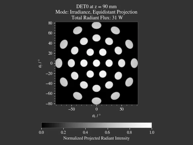
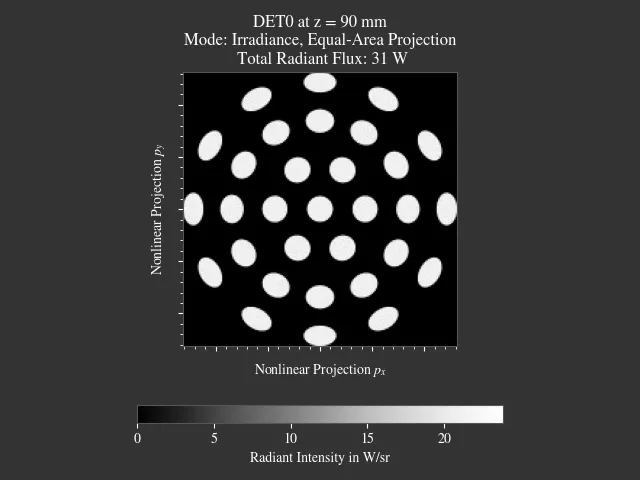
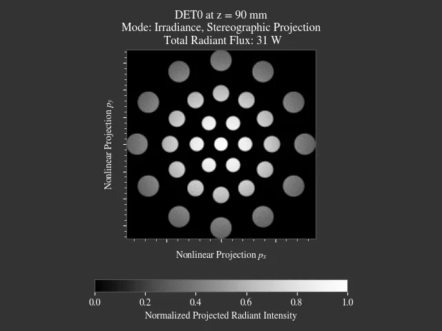
4.8.6. Sphere Projections

With a spherical detector surface, there are multiple ways to project it down to a rectangular surface. Note that there is no possibility to correctly represents angles, distances and areas at the same time.

Below you can find the projection methods implemented in optrace and links to a more detailed explanation. Details on the math applied are found in the math section in Section 5.4.2.

The available methods are:

"Orthographic"	Perspective projection, sphere surface seen from far away [1]
"Stereographic"	Conformal projection (preserving local angles and shapes) [2]
"Equidistant"	Projection keeping the radial direction from a center point equal [3]
"Equal-Area"	Area preserving projection [4]

Table 4.7 Tissot’s indicatrices for different projection methods. All circles should have the same size, shape and brightness. Taken from the Sphere Projections example

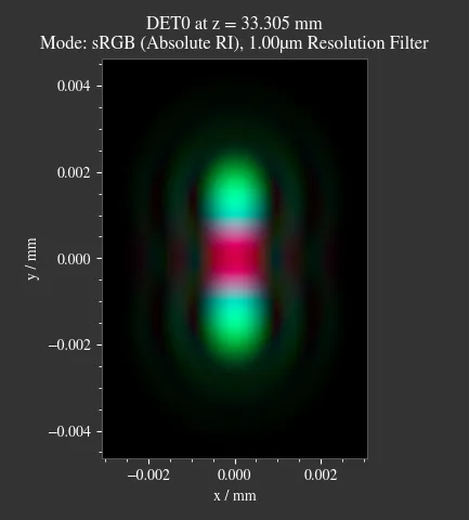
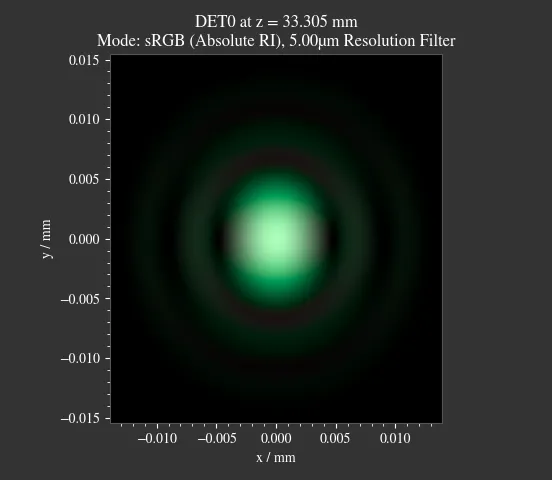
4.8.7. Resolution Limit Filter

Unfortunately, optrace does not take wave optics into account when simulating. To estimate the effect of a resolution limit the RenderImage class provides a limit parameter. For a given limit value a corresponding Airy disc is created, that is convolved with the image. This parameter describes the Rayleigh limit, being half the size of the Airy disc core (zeroth order), known from the equation:

(4.21)\[r = 0.61 \frac{\lambda}{\text{NA}}\]

Where \(\lambda\) is the wavelength and \(\text{NA}\) is the numerical aperture. While the limit is wavelength dependent, one fixed value is applied to all wavelengths for simplicity. Only the first two diffraction orders (core + 2 rings) are used, higher orders should have a negligible effect.

Note

The limit parameter is only an estimation of how large the impact of a resolution limit on the image is.

The simulation neither knows the actual limit nor takes into interference and diffraction.

Table 4.8 Images of the focus in the Achromat example. From left to right: No filter, filter with 1 µm size, filter with 5 µm size. For a setup with a resolution limit of 5 µm we are clearly inside the limit, but even for 1 µm we are diffraction limited.

The limit parameter can be applied while either creating the RenderImage (ot.RenderImage(..., limit=5)) or by providing it to methods the create an RenderImage (Raytracer.detector_image(..., limit=1), Raytracer.iterative_render(..., limit=2.5).

4.8.8. Generating Images from RenderImage

Usage

From a RenderImage multiple image modes can be generated with the get method. The function takes an optional pixel size parameter, that determines the pixel count for the smaller image size. Internally the RenderImage stores its data with a pixel count of 945 for the smaller side, while the larger side is either 1, 3 or 5 times this size, depending on the side length ratio. Therefore no interpolation takes place that would falsify the results. To only join full bins, the available sizes are reduced to:

>>> ot.RenderImage.SIZES
[1, 3, 5, 7, 9, 15, 21, 27, 35, 45, 63, 105, 135, 189, 315, 945]

As can be seen, all sizes are integer factors of 945. All sizes are odd, so there is always a pixel/line/row for the image center. Without a center pixel/line/row the center position would be badly defined, either being offset or jumping around depending on numerical errors.

In the function get the nearest value from RenderImage.SIZES to the user selected value is chosen. Let us assume the dimg has a side length of s=[1, 2.63], so it was rendered in a resolution of 945x2835. This is the case because the nearest side factor to 2.63 is 3 and because 945 is the size for all internally rendered images. From this resolution the image can be scaled to 315x945 189x567 135x405 105x315 63x189 45x135 35x105 27x81 21x63 15x45 9x27 7x21 5x15 3x9 1x3. The user image is then scaled into size 315x945, as it is the nearest to a size of 500.

These restricted pixel sizes lead to typically non-square pixels. But these are handled correctly by plotting and processing functions. They will only become relevant when exporting the image to an image file, where the pixels must be square. More details are available in section Section 4.8.11.

To get a Illuminance image with 315 pixels we can write:

img = dimg.get("Illuminance", 500)

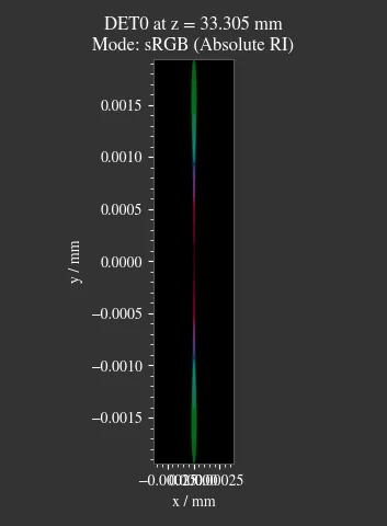
Only for image modes "sRGB (Perceptual RI)" and "sRGB (Absolute RI)" the returned object type is RGBImage . For all other modes it is of type ScalarImage.

For mode "sRGB (Perceptual RI)" there are two optional additional parameters L_th and chroma_scale. See Section 4.15.5 for more details.

Image Modes

"Irradiance"	Image of power per area
"Illuminance"	Image of luminous power per area
"sRGB (Absolute RI)"	A human vision approximation of the image. Colors outside the gamut are chroma-clipped. Preferred sRGB-Mode for “natural”/”everyday” scenes.
"sRGB (Perceptual RI)"	Similar to sRGB (Absolute RI), but with uniform chroma-scaling. Preferred mode for scenes with monochromatic sources or highly dispersive optics.
"Outside sRGB Gamut"	Pixels outside the sRGB gamut are shown in white
"Lightness (CIELUV)"	Human vision approximation in greyscale colors. Similar to Illuminance, but with non-linear brightness function.
"Hue (CIELUV)"	Hue image from the CIELUV colorspace
"Chroma (CIELUV)"	Chroma image from the CIELUV colorspace. Depicts how colorful an area seems compared to a similar illuminated grey area.
"Saturation (CIELUV)"	Saturation image from the CIELUV colorspace. How colorful an area seems compared to its brightness. Quotient of Chroma and Lightness.

The difference between chroma and saturation is more thoroughly explained in [5]. An example for the difference of both sRGB modes is seen in Table 5.5.

Table 4.9 Renderes images from the Image Render example. From left to right, top to bottom: sRGB (Absolute RI), sRGB (Perceptual RI), Outside sRGB Gamut, Lightness, Irradiance, Illuminance, Hue, Chroma, Saturation.

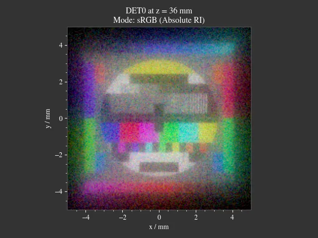
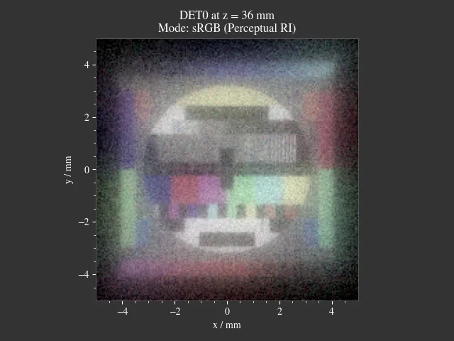
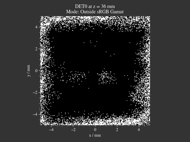
Fig. 4.32 sRGB Absolute RI	Fig. 4.33 sRGB Perceptual RI	Fig. 4.34 Values outside of sRGB
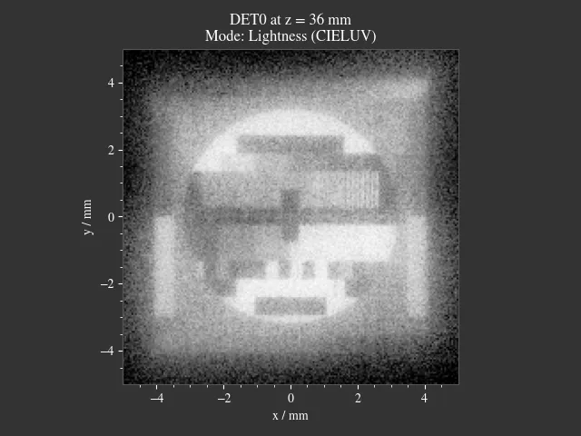
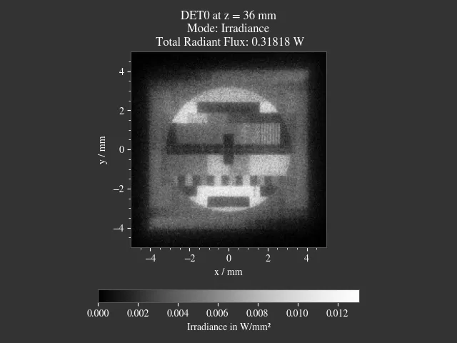
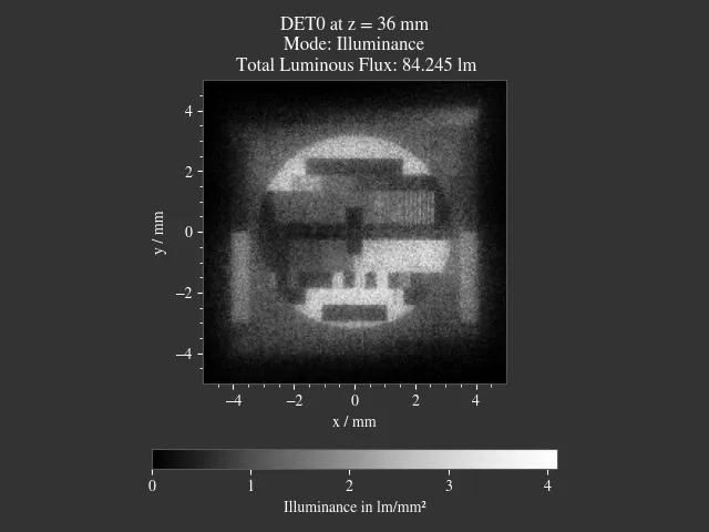
Fig. 4.35 Lightness (CIELUV)	Fig. 4.36 Irradiance	Fig. 4.37 Illuminance
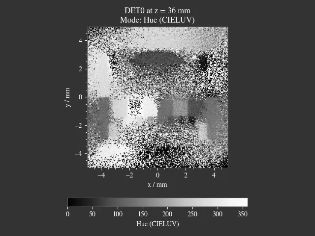
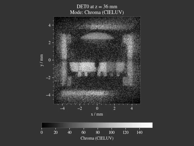
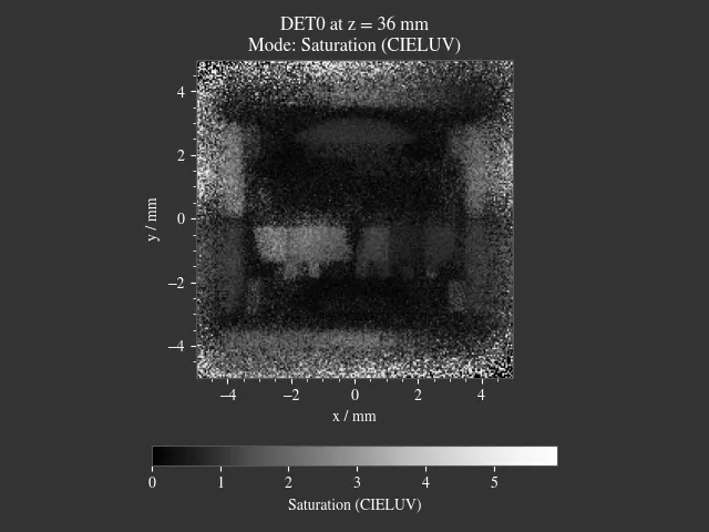
Fig. 4.38 Hue (CIELUV)	Fig. 4.39 Chroma (CIELUV)	Fig. 4.40 Saturation (CIELUV)

4.8.9. Converting between GrayscaleImage and RGBImage

Use RGBImage.to_grayscale_image() to convert a colored RGBImage to a grayscale image. The channels are weighted according to their luminance, see question 9 of [6]. Use GrayscaleImage.to_rgb_image() to convert a GrayscaleImage to an RGB image. All grayscale values are repeated for the R, G, B channels. Both methods require no parameters and return the other image object type.

4.8.10. Image Profile

An image profile is a line profile of a generated image in x- or y-direction. It is created by the profile() method. The parameters x and y define the positional value for the profile.

The following example generates an image profile in y-direction at x=0:

bins, vals = img.profile(x=0)

For a profile in x-direction we can write:

bins, vals = img.profile(y=0.25)

The function returns a tuple of the histogram bin edges and the histogram values, both one dimensional numpy arrays. Note that the bin array is larger by one element.

4.8.11. Saving Images

ScalarImage and RGBImage can be saved to disk in the following way:

img.save("image_render_srgb.jpg")

The file type is automatically determined from the file ending in the path string.

Often times the image is flipped, but it can be flipped using flip=True. This rotates the image by 180 degrees.

img.save("image_render_srgb.jpg", flip=True)

Depending on the file type ,there can be additional saving parameters provided, for instance compression settings:

import cv2
img.save("image_render_srgb.jpg", params=[cv2.IMWRITE_PNG_COMPRESSION, 1], flip=True)

See cv2.ImwriteFlags for more information. The image is automatically interpolated so the exported image has the same side length ratio as the RGBImage or ScalarImage object.

Note

While the Image has arbitrary, generally non-square pixels, for the export the image is rescaled to have square pixels. However, in many cases there is no exact ratio that matches the side ratio with integer pixel counts. For instance, an image with sides 12.532 x 3.159 mm and a desired export size of 105 pixels for the smaller side leads to an image of 417 x 105 pixels. This matches the ratio approximately, but is still off by -0.46 pixels (around -13.7 µm). This error gets larger the smaller the resolution is.

4.8.12. Plotting Images

See Plotting Images.

4.8.13. Image Properties

Overview

Classes ScalarImage, RenderImage, RGBImage share property methods. These include geometry information and metadata. When a ScalarImage or RGBImage is created from a RenderImage, the metadata and geometry is automatically propagated into the new object.

Size Properties

>>> dimg.extent
array([-0.0081,  1.0081, -0.0081,  1.0081])

>>> dimg.s[1]
1.0162

The data shape:

>>> dimg.shape
(945, 945, 4)

Apx is the area per pixel in mm²:

>>> dimg.Apx
1.1563645362671817e-06

Metadata

>>> dimg.limit
3.0

>>> dimg.projection is None
True

Data Access

Access the underlying array data using:

dimg.data

Image Powers (RenderImage only)

Power in W and luminous power in lm:

dimg.power()
dimg.luminous_power()

Image Mode (RGBImage/GrayscaleImage/ScalarImage only)

>>> img.quantity
'Illuminance'

4.8.14. Image Presets

Below you can find different images presets. As for the image classes, a specification of either the s or extent geometry parameter is mandatory. One possible call could be:

img = ot.presets.image.cell(s=[0.2, 0.3])

Table 4.10 Photos of natural scenes or objects

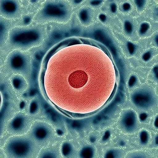
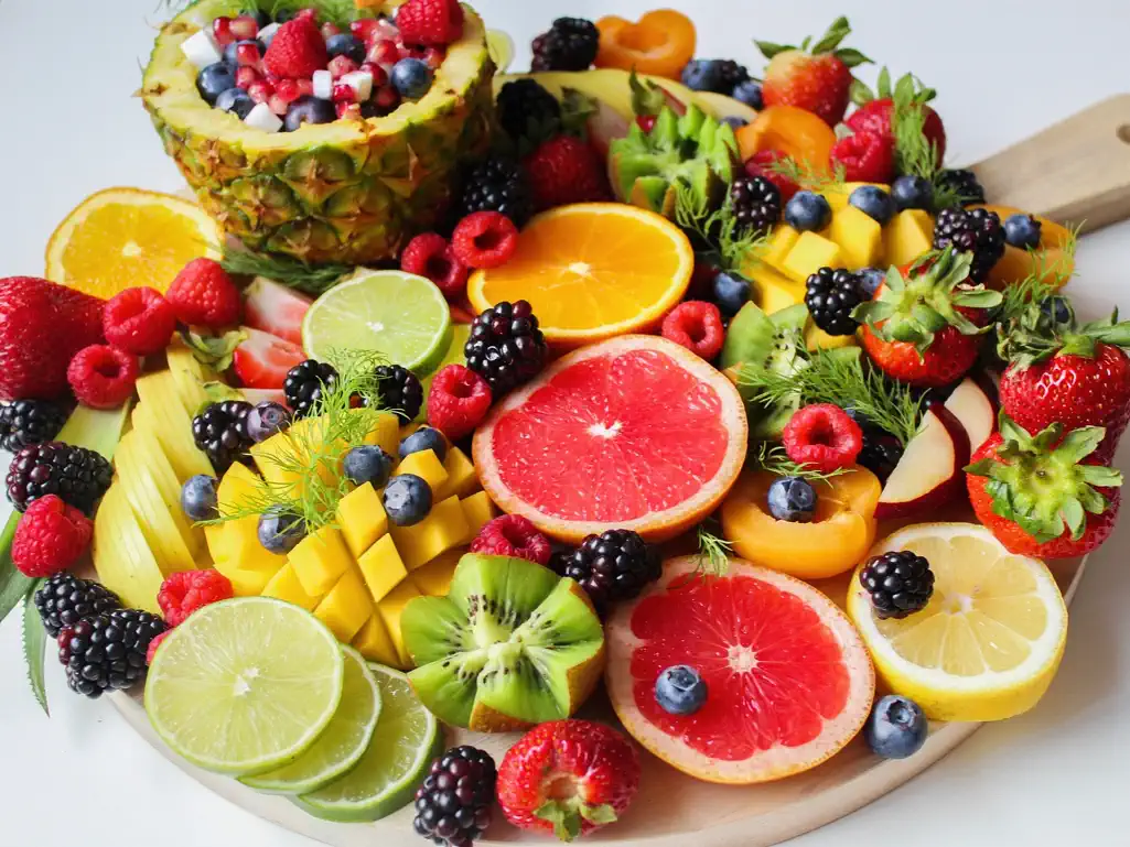
Fig. 4.41 Cell image for microscope examples (Source). Usable as ot.presets.image.cell.	Fig. 4.42 Photo of different fruits on a tray (Source). Usable as ot.presets.image.fruits.
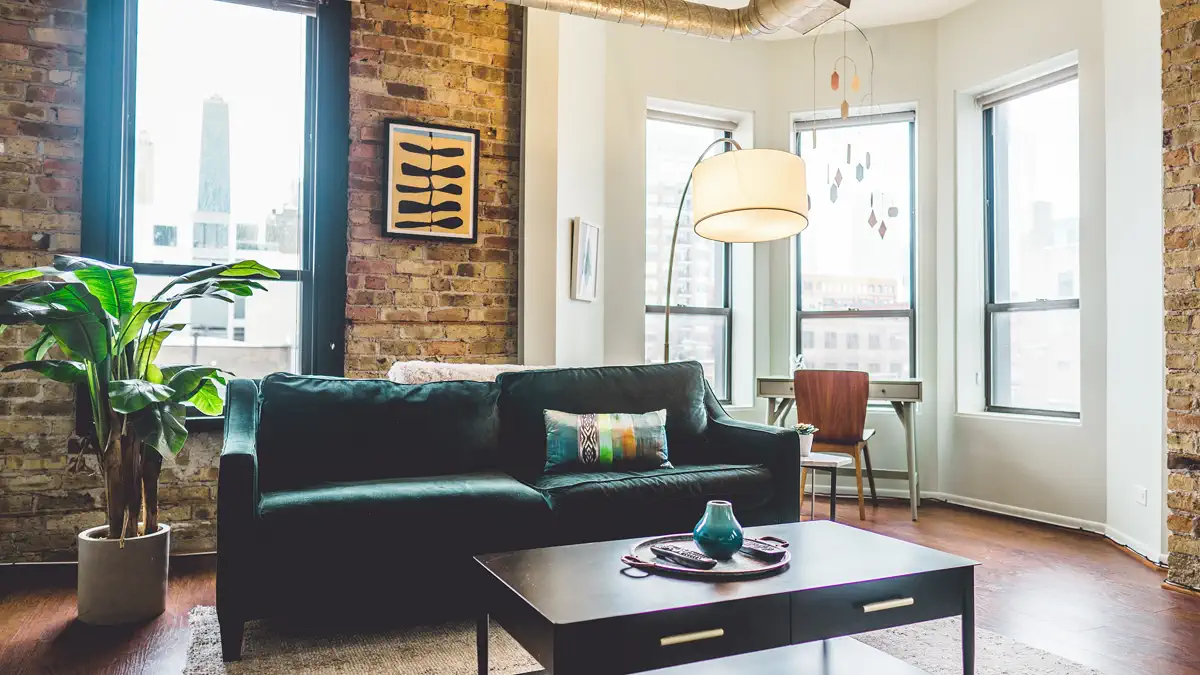
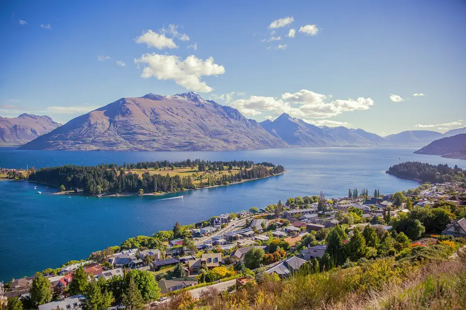
Fig. 4.43 Green sofa in an interior room (Source). Usable as ot.presets.image.interior	Fig. 4.44 Landscape image of a mountain and water scene (Source). Usable as ot.presets.image.landscape
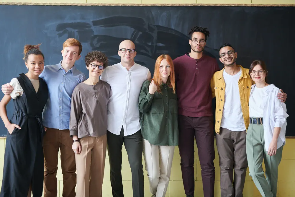
Fig. 4.45 Photo of a keyboard and documents on a desk (Source). Usable as ot.presets.image.documents.	Fig. 4.46 Photo of a group of people in front of a blackboard (Source). Usable as ot.presets.image.group_photo
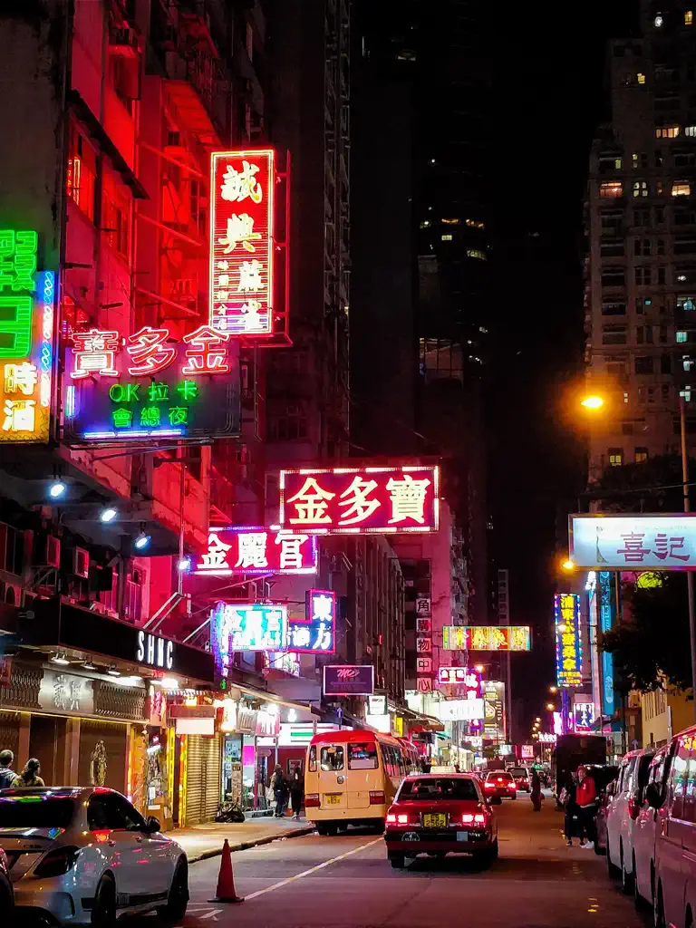
Fig. 4.47 Photo of a Hong Kong street at night (Source). Usable as ot.presets.image.hong_kong.

Table 4.11 Test images for color, resolution or distortion. The ETDRS chart images, Siemens star and grid methods return GrayscaleImage, all other images RGBImage.

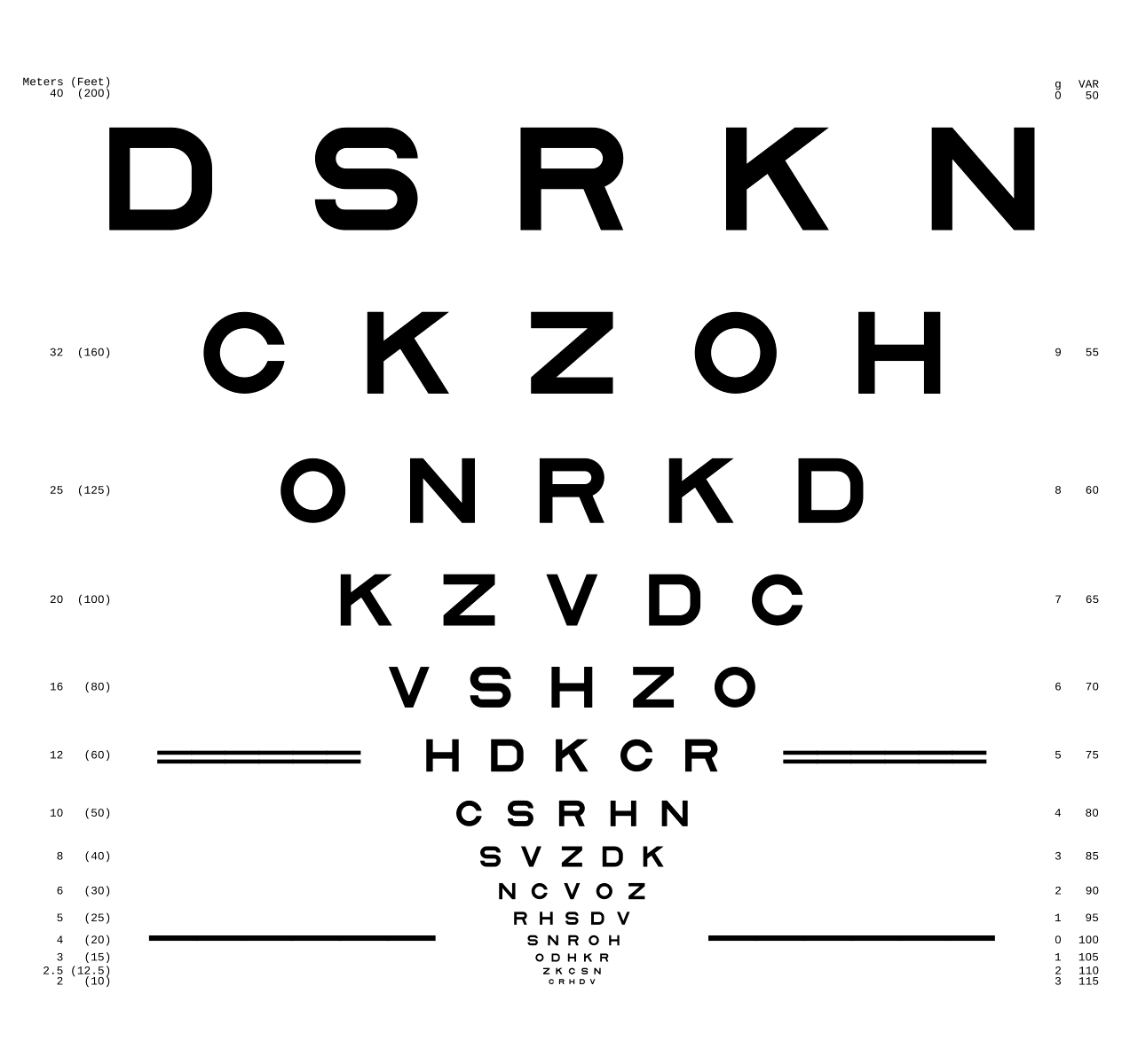
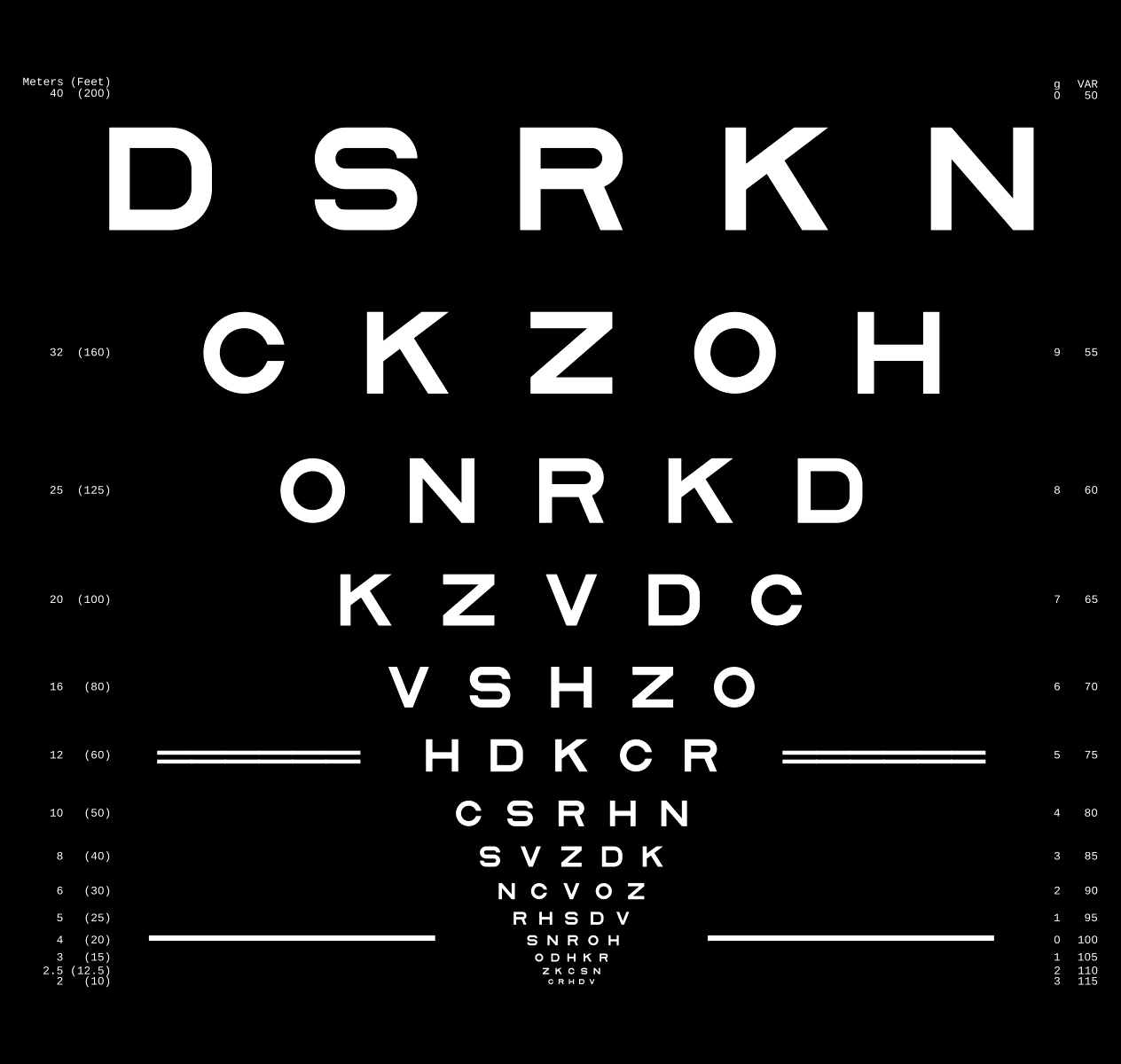
Fig. 4.48 ETDRS Chart standard (Source). Usage with ot.presets.image.ETDRS_chart.	Fig. 4.49 ETDRS Chart standard. Edited version of the ETDRS image. Usage with ot.presets.image.ETDRS_chart_inverted
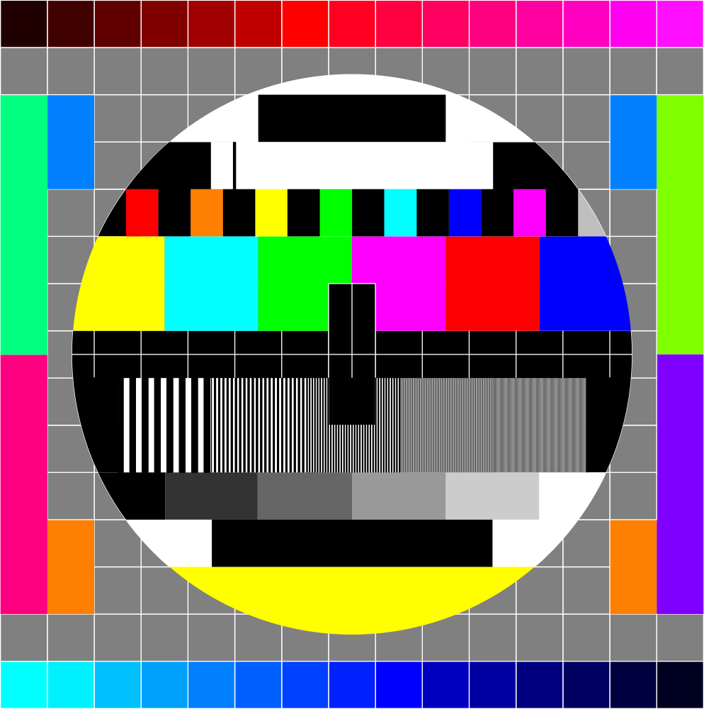
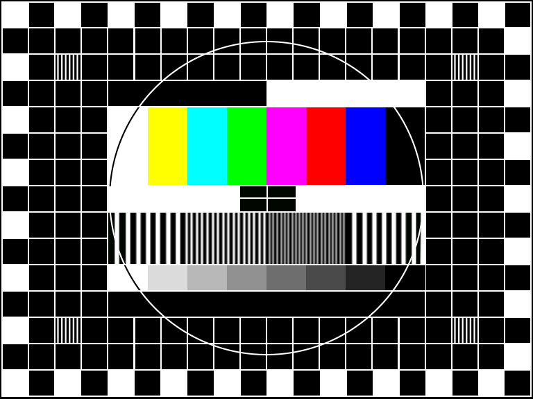
Fig. 4.50 TV test card #1 (Source). Usage with ot.presets.image.tv_testcard1	Fig. 4.51 TV test card #2 (Source). Usage with ot.presets.image.tv_testcard2
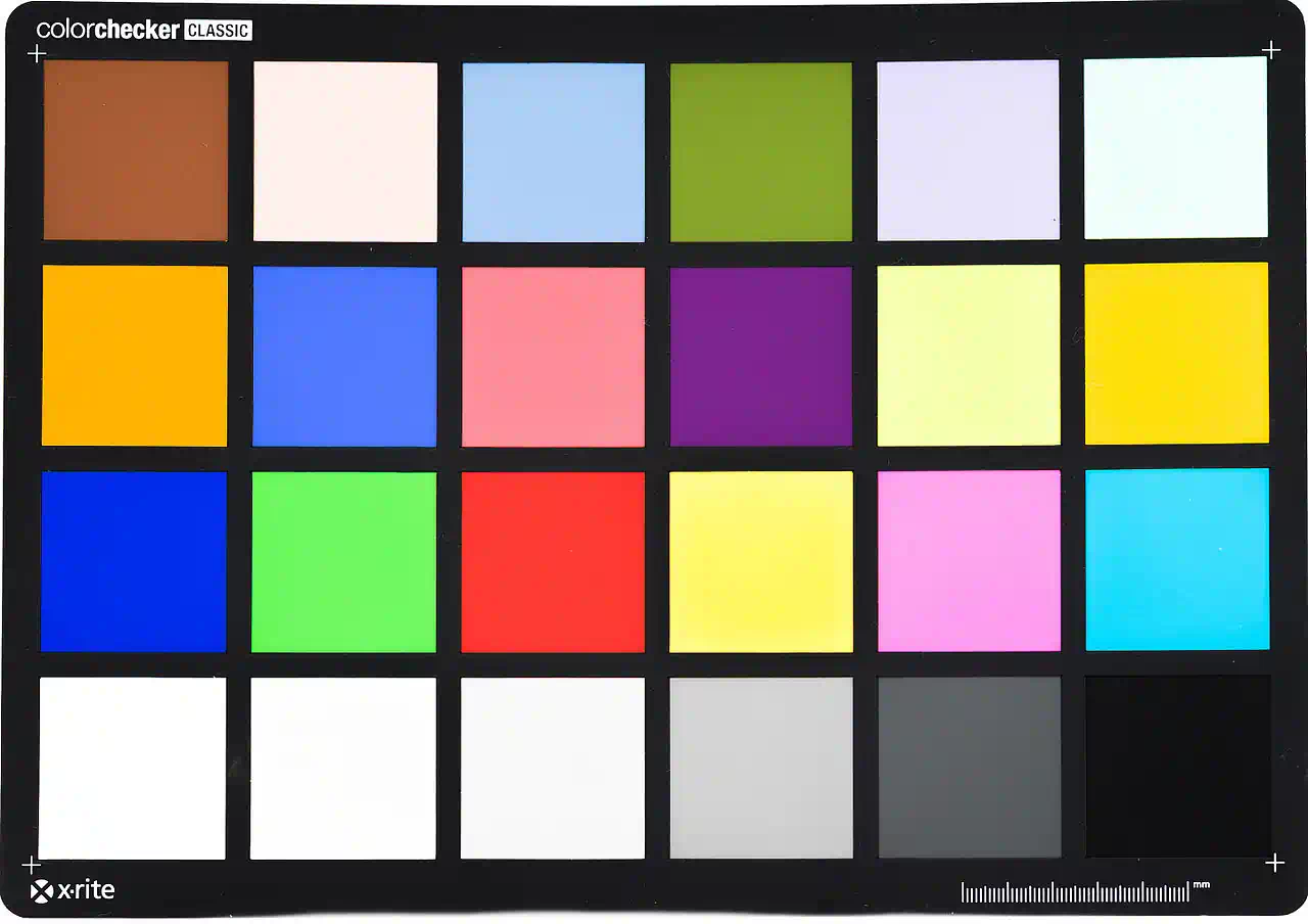
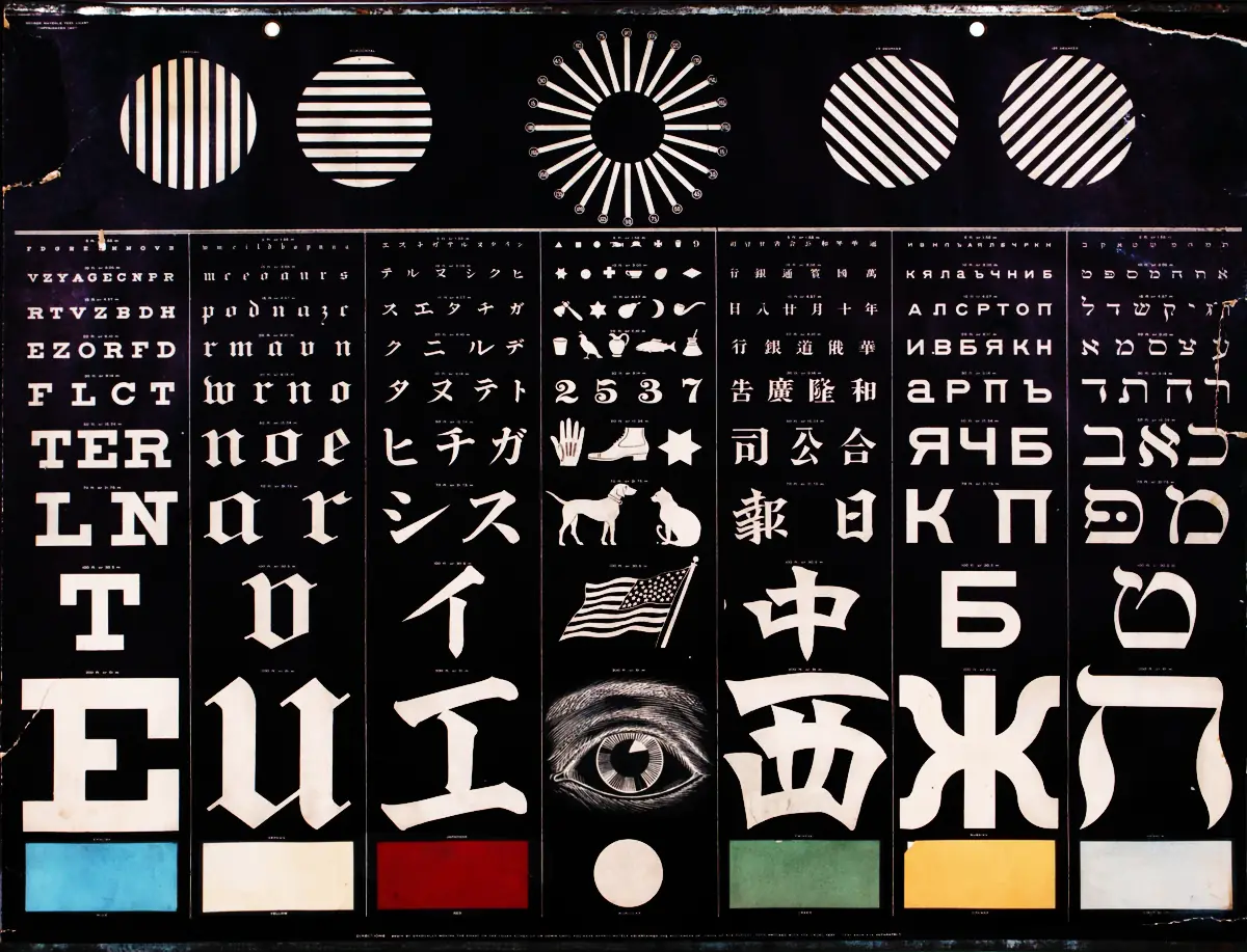
Fig. 4.52 Color checker chart (Source). Usage with ot.presets.image.color_checker	Fig. 4.53 Photo of a vintage eye test chart (Source). Usage with ot.presets.image.eye_test_vintage.
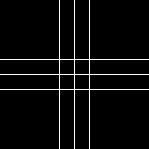
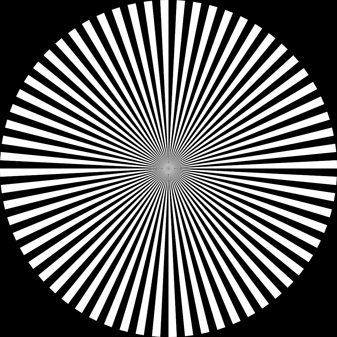
Fig. 4.54 White grid on black background with 10x10 cells. Useful for distortion characterization. Own creation. Usage with ot.presets.image.grid	Fig. 4.55 Siemens star image. Own creation. Usage with ot.presets.image.siemens_star

---

References

[1]

Wikipedia. Orthographic map projection. 2022. URL: https://en.wikipedia.org/wiki/Orthographic_map_projection (visited on 2022-12-01).

[2]

Wikipedia. Stereographic map projection. 2022. URL: https://en.wikipedia.org/wiki/Stereographic_map_projection (visited on 2022-12-01).

[3]

Wikipedia. Azimuthal equidistant projection. 2022. URL: https://en.wikipedia.org/wiki/Azimuthal_equidistant_projection (visited on 2022-12-01).

[4]

Wikipedia. Lambert azimuthal equal-area projection. 2022. URL: https://en.wikipedia.org/wiki/Lambert_azimuthal_equal-area_projection (visited on 2022-12-01).

[5]

David Briggs. The difference between chroma and saturation. 2016. URL: https://munsell.com/color-blog/difference-chroma-saturation/ (visited on 2023-01-03).

[6]

Charles Poynton. Frequently asked questions about color. 1997. URL: https://poynton.ca/PDFs/ColorFAQ.pdf (visited on 2025-03-26).