4.4. Geometry Groups

4.4.1. Group

4.4.1.1. Overview

A Group is a container of several elements.

It contains the following functionality:

Functionality	Example
Adding and removing one or more elements:	G.add(obj) G.remove(obj)
Emptying all elements:	G.clear()
check if an element is included:	G.has(obj)
move all elements at once:	G.move_to([5.3, 0.0, 12.3])
rotate or flip all elements:	G.rotate(-12) G.flip()
create a ray transfer matrix of the whole group:	G.tma()

A Group object stores all elements in their own class lists: lenses, ray_sources, detectors, markers, filters, apertures, volumes. Where IdealLens and Lens are included in the same list, all marker types are included in markers and all volume types in volumes.

When adding objects, the order of objects remains the same. Thus lenses[2] denotes the lens that was added third (counting starts at 0). For clarity, it is recommended to add objects in their correct z-order.

4.4.1.2. Geometry properties

A group shares the same functions for geometry properties and manipulations as an element, see Shared Functions/Properties. There are three main differences:

Position

The position property describes the position of the first element (smallest z-position).

Flipping

When flipping, additional parameters y0, z0 can be provided to define a rotation axis. By default, y0 = 0 and z0 are the center of the extent of the group. See Group.flip for details.

Rotation

For rotation, parameters x0, y0 can be additionally provided, which also describe a position of the rotation axis. By default, both are zero. See Group.rotate.

4.4.1.3. Example

The following example creates a Group consisting of an IdealLens and an Aperture.

IL = ot.IdealLens(r=6, D=-20, pos=[0, 0, 10])
F = ot.Aperture(ot.RingSurface(ri=0.5, r=10), pos=[0, 0, 30])

G = ot.Group([IL, F])

Next, we flip the group, reversing the z-order of the elements and flipping each element around its x-axis through the center. Since all elements are rotationally symmetric, this just reorders them. After flipping we move the group to a new position. This position is the new position for the first element (which after flipping is the filter), whereas all relative distances to all other elements are kept equal.

G.flip()
G.move_to([0, 1, 0])

The filter is the first element and has the same position as we moved the group to.

>>> G.apertures[0].pos
array([0., 1., 0.])

The lens has the same relative distance of \(\Delta z = 20\) mm relative to the Filter, but in a different absolute position and now behind the filter.

>>> G.lenses[0].pos
array([ 0.,  1., 20.])

4.4.2. Loading ZEMAX OpticStudio Geometries (.zmx)

It is possible to load .zmx geometries into optrace. The following example loads a geometry from file setup.zmx into the raytracer:

RT = ot.Raytracer(outline=[-20, 20, -20, 20, -20, 200])

RS = ot.RaySource(ot.CircularSurface(r=0.05),
                  spectrum=ot.presets.light_spectrum.d65,
                  pos=[0, 0, -10])
RT.add(RS)

n_schott = ot.load_agf("schott.agf")
G = ot.load_zmx("setup.zmx", n_dict=n_schott)
RT.add(G)

RT.trace(10000)

For the materials to be loaded correctly all mentioned names in the .zmx file need to be included in the n_dict dictionary. You can either load them from a .agf catalogue like in Section 4.6.4 or create the dictionary manually.

A list of exemplary .zmx files can be found in the following repository.

Unfortunately, the support is only experimental, as there is no official documentation on the file format. Additionally, only a subset of all ZEMAX OpticStudio functionality is supported, including:

• SEQ-mode only

• UNIT must be MM

• only STANDARD or EVENASPH surfaces, this is equivalent to RingSurface, CircularSurface, SphericalSurface, ConicSurface, AsphericSurface in optrace

• no support for coatings

• temperature or absorption behavior of the material is neglected

• only loads lens and aperture geometries, no support for additional objects

Information on the file format can be found in [1], as well as here and here.

4.4.3. Geometry Presets

4.4.3.1. Ideal Camera

An ideal camera preset is included, that provides aberration-free imaging towards a detector.

The preset is loaded with ot.presets.geometry.ideal_camera and returns a Group object consisting of a lens and a detector. Required parameters are the object position z_g as well as the camera position (the position of the lens) cam_pos, as well as the image distance b, which in this case is just the difference distance between lens and detector. A visual presentation of these quantities is shown in the figure below.

An exemplary call could be:

G = ot.presets.geometry.ideal_camera(cam_pos=[1, -2.5, 12.3],
                                     z_g=-56.06, b=10)

The lens diameter parameter r and detector radius r_det are provided by doing the following:

G = ot.presets.geometry.ideal_camera(cam_pos=[1, -2.5, 12.3],
                                     z_g=-56.06, b=10, r=5, r_det=8)

The function also supports an infinite position of z_g = -np.inf.

When given a desired object magnification \(m\), the image distance parameter \(b\) can be calculated with:

(4.3)\[m = \frac{b}{g} \Rightarrow b = m \cdot g\]

Which should be known from the fundamentals of optics. Where \(g\) is the object distance, in our example z_g - cam_pos[2]. Note that \(b, g\) both need to be positive for this preset to work.

Fig. 4.17 Visualization of the ideal_camera parameters.

4.4.3.2. LeGrand Paraxial Eye Model

The LeGrand full theoretical eye model is a simple model consisting of only spherical surfaces and wavelength-independent refractive indices. It models the paraxial behavior of a far-adapted eye.

Table 4.2 LeGrand Full Theoretical Eye Model [2]

Surface	Radius in mm	Conic Constant	Refraction Index to next surface	Thickness (mm) (to next surface)
Cornea Anterior	7.80	0	1.3771	0.5500
Cornea Posterior	6.50	0	1.3374	3.0500
Lens Anterior	10.20	0	1.4200	4.0000
Lens Posterior	-6.00	0	1.3360	16.5966
Retina	-13.40	0	-	-

The preset legrand_eye is located in ot.presets.geometry and is called as a function. It returns a Group object that can be added to a Raytracer. Provide a pos parameter to position it at an other position than [0, 0, 0].

RT = ot.Raytracer(outline=[-10, 10, -10, 10, -10, 60])
eye_model = ot.presets.geometry.legrand_eye(pos=[0.3, 0.7, 1.2])
RT.add(eye_model)

Optional parameters include a pupil diameter and a lateral detector (retina) radius, both provided in millimeters.

eye_model = ot.presets.geometry.legrand_eye(pupil=3, r_det=10, pos=[0.3, 0.7, 1.2])

4.4.3.3. Arizona Eye Model

A more advanced model is the arizona_eye model, which tries to match clinical levels of aberration for different adaption levels. It consists of conic surfaces, dispersive media and adaptation dependent parameters.

Table 4.3 Arizona Eye Model [2]

Surface	Radius in mm	Conic Constant	Refraction Index to next surface	Abbe Number	Thickness (mm) (to next surface)
Cornea Anterior	7.80	-0.25	1.377	57.1	0.55
Cornea Posterior	6.50	-0.25	1.337	61.3	\(t_\text{aq}\)
Lens Anterior	\(R_\text{ant}\)	\(K_\text{ant}\)	\(n_\text{lens}\)	51.9	\(t_\text{lens}\)
Lens Posterior	\(R_\text{post}\)	\(K_\text{post}\)	1.336	61.1	16.713
Retina	-13.40	0	-	-	-

With an accommodation level \(A\) in dpt the missing parameters are calculated using: [2]

(4.4)\[\begin{split}\begin{array}{ll} R_{\text {ant }}=12.0-0.4 A & K_{\text {ant }}=-7.518749+1.285720 A \\ R_{\text {post }}=-5.224557+0.2 A & K_{\text {post }}=-1.353971-0.431762 A \\ t_{\text {aq }}=2.97-0.04 A & t_{\text {lens }}=3.767+0.04 A \\ n_{\text {lens }}=1.42+0.00256 A-0.00022 A^2 \end{array}\end{split}\]

Accessing and adding the group works the same as for the legrand_eye preset.

RT = ot.Raytracer(outline=[-10, 10, -10, 10, -10, 60])
eye_model = ot.presets.geometry.arizona_eye(pos=[0.3, 0.7, 1.2])
RT.add(eye_model)

As for the legrand_eye, we have the parameters pupil and r_det. Additionally there is an adaptation parameter specified in diopters, which defaults to 0 dpt.

eye_model = ot.presets.geometry.arizona_eye(adaptation=1, pupil=3, r_det=10, pos=[0.3, 0.7, 1.2])

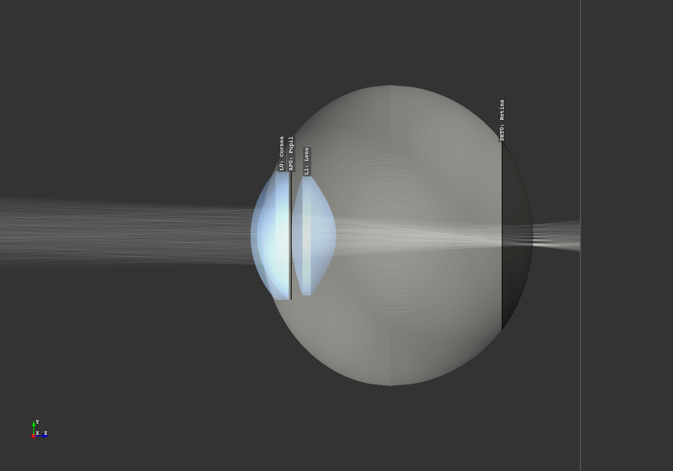
Fig. 4.18 Eye model in the Arizona Eye Model example script.

---

References

[1]

Focus Software, Incorporated. Zemax® optical design program user’s guide version 9.0, chapter 29: the zmx file format. 2000. URL: https://pdfcoffee.com/zemaxmanual-pdf-free.html (visited on 2024-04-09).

[2] (1,2,3)

Jim Schwiegerling. Field Guide to Visual and Ophthalmic Optics. SPIE, 2004. URL: https://doi.org/10.1117/3.592975, doi:10.1117/3.592975.