4.11. PSF Convolution
4.11.1. Overview
Convolution significantly speeds up image formation by parallelizing the effect of the PSF (point spread function) for every object point. This results in a nearly sampling noise-free image in a small fraction of the time normally required for raytracing. A PSF is nothing different than the impulse response of the optical system for the given object and image distance combination. It changes spatially, but for a small angular range it can be assumed constant. However, this also implies that many aberration can’t be simulated with this approach, including astigmatism, coma, vignette, and distortion.
The convolution approach in optrace requires:
the image and its size parameters
the PSF and its size parameters
a magnification factor
optional parameters for padding and slicing
optional parameters for the output color conversion
Both colored input images and color PSFs are supported. However, there are some limitations and restrictions, that will be illustrated next. See the details in section Section 5.6.1 for even more technical information.
4.11.2. Grayscale and color image convolution
A call to convolve requires the image and PSF as arguments.
Generally, the convolution must be done on a per-wavelength basis to be physically correct, as each wavelength
has their own PSF. See the details in section Section 5.6.1.
However, there are special cases, where this is not required. One import term will be spectral homogenity which describes an object that emits the same spectrum at all locations, only differing by an intensity factor. Such objects have a single hue and saturation color, differing only in its brightness. Note that that the inverse is not true, objects with the same color don’t necessarily mean a spectral homogeneous object, as multiple spectra can produce the same color impression.
As mentioned in section Section 4.7.1, values of the pixels of the RGBImage and GrayscaleImage
are not linear to the physical intensities of the color, but scaled non-linearly to account for the human perception.
The convolve converts the images to linear values and does the convolution
on these linear color space coordinates. At the end, the linear image is converted back
to a RGBImage or GrayscaleImage.
Grayscale Image and Grayscale PSF
The typical case of grayscale-grayscale convolution is for a black-and-white image and colorless, wavelength-independent PSF:
img = ot.presets.image.grid([1, 1]) #  type GrayscaleImage
psf = ot.presets.psf.airy(8)  # type GrayscaleImage
img2 = ot.convolve(img, psf)  # type GrayscaleImage
However, this also works for a more general case: Spectral homogeneous image and spectral homogeneous PSF. For instance, this is also true for a intensity distribution emitting a blue spectrum everywhere, and a PSF that has a single spectrum at all locations. It doesn’t need to be the same spectrum as the source image. For instance, the PSF can include violet wavelengths only, because the optical system absorbed the more blueish wavelengths of the spectrum.
To model this, simulate and render a PSF by creating a point source with the desired image spectrum.
Then convert both the image and the PSF to a GrayscaleImage and convolve them.
The result is also a GrayscaleImage, showing the intensity distribution.
# raytracer
RT = ot.Raytracer(...)

# create R, G, B sRGB primary spectra with the correct power ratios
# create image spectrum and point source
my_spectrum = ot.LightSpectrum(...)
RS = ot.RaySource(ot.Point(), spectrum=my_spectrum, pos=...)
RT.add(RS)

# add more geometries and detector
...

# trace
RT.trace(10000)

# render detector image
psf = RT.detector_image()
psf_srgb = psf.get("sRGB (Absolute RI)")  # convert RenderImage to sRGB
psf_gray = psf_srgb.to_grayscale_image()  # convert sRGB to grayscale

# convolve
img_gray = ot.Grayscale(...)  # image emitting my_spectrum
img2 = ot.convolve(img_gray, psf_gray, ...)
The physical interpretation is that the image emits the source spectrum my_spectrum according to
the spatial distribution given by img_gray and the resulting image emits the spectrum at the detector with
spatial intensity given by img2.
You can calculate the detector spectrum from the PSF:
# detector image spectrum
img_spec = RT.detector_spectrum()
Colored Image and grayscale PSF
Here, the image is of type RGBImage and the PSF is wavelength-independent, given as GrayscaleImage.
Internally, each R, G, B channel is convolved separately with the PSF and the result is also an RGBImage.
img = ot.presets.image.fruits([0.3, 0.4]) #  type RGBImage
psf = ot.presets.psf.airy(8)  # type GrayscaleImage
img2 = ot.convolve(img, psf)  # type RGBImage
This is only viable when the optical system treats all wavelengths equally, with no chromatic effects such as dispersion or wavelength-dependent absorption.
Grayscale Image and colored PSF
This convolution type implies a spectral homogeneous image and a colored PSF.
The image is a GrayscaleImage representing the human visible intensities.
The PSF has to be a RenderImage to includes all human visible colors
and must be rendered for the desired source spectrum.
If the image should emit a D65 spectrum, it should be traced and rendered with the D65 spectrum.
If it should emit a blue spectrum, it should be traced and rendered with the same blue spectrum.
Doing so, the color information is included in the PSF and will be applied in the convolution operation.
The result is an RGBImage.
# raytracer
RT = ot.Raytracer(...)

# create R, G, B sRGB primary spectra with the correct power ratios
# create image spectrum and point source
my_spectrum = ot.LightSpectrum(...)
RS = ot.RaySource(ot.Point(), spectrum=my_spectrum, pos=...)
RT.add(RS)

# add more geometries and detector
...

# trace
RT.trace(10000)

# render detector image
psf = RT.detector_image()

# convolve
img_gray = ot.Grayscale(...)
# ^-- spatial distribution emitting "my_spectrum" defined above
img2 = ot.convolve(img_gray, psf, ...)
Colored Image and colored PSF
Colored image and PSF are only viable in one special case: The image is simulated as emitting a combination of R, G, B sRGB primary spectra for each pixel. And three PSFs were rendered for each R, G, B primary with the correct power ratios. Only then will the convolution approach be correct.
Without this restriction, there are infinitely many solutions, as many spectra can produce the same sRGB color and each spectrum produces slightly different PSFs. This solution, assuming a composition of sRGB primary spectra, will then be just one of many.
The input image is a RGBImage, while the PSF is provided as a three-element list of R, G, B RenderImage.
As described above, they need to be rendered with a specific spectrum and power and the images need to have the same
size. Without the power factors, the white balance will be incorrect.
Below you can find an example for doing things correctly.
# raytracer
RT = ot.Raytracer(...)

# create R, G, B sRGB primary spectra with the correct power ratios
RS_args = dict(surface=ot.Point(), pos=[0, 0, 0], ...)
RS_R = ot.RaySource(**RS_args, spectrum=ot.presets.light_spectrum.srgb_r,
                    power=ot.presets.light_spectrum.srgb_r_power_factor)
RS_G = ot.RaySource(**RS_args, spectrum=ot.presets.light_spectrum.srgb_g,
                    power=ot.presets.light_spectrum.srgb_g_power_factor)
RS_B = ot.RaySource(**RS_args, spectrum=ot.presets.light_spectrum.srgb_b,
                    power=ot.presets.light_spectrum.srgb_b_power_factor)
RT.add([RS_R, RS_G, RS_B)

# add more geometries and detector
...

# trace
RT.trace(10000)

# render detector images, index 0 is R, index 1 is G, index 2 is B
psf0 = RT.detector_image()  # needed so we know the approximate spatial image extent using psf0.extent
psf_r = RT.detector_image(source_index=0, extent=psf0.extent)
psf_g = RT.detector_image(source_index=1, extent=psf0.extent)
psf_b = RT.detector_image(source_index=2, extent=psf0.extent)
psf_rgb = [psf_r, psf_g, psf_b]

# convolve
img = ot.presets.image.color_checker([1, 1])
img2 = ot.convolve(img, psf_rgb, ...)
4.11.3. Restrictions
convolution is done on supported image classes only
the implementation prohibits convolving two
RGBImageor twoRenderImageimage and PSF resolutions must lie between 50x50 pixels and 4 megapixels
the PSF needs to be at least twice as large as the scaled input image (image scaled with the magnification factor)
when convolving two colored images, the resulting image is only one possible solution of many
when R, G, B
RenderImageare provided for polychromatic convolution, they all need to have the same spatial extentscipy.signal.fftconvolve()is involved, so small numerical errors can appear in dark image regions
The convolution function does not check if the convolution of the underlying image is reasonable physically. There are no checks whether both images represent the same underlying physical quantity or possess a linear spatial geometry (e.g not being a sphere projections).
4.11.4. Additional Function Parameters
Magnification Factor
The magnification factor is equivalent the magnification factor derived from geometrical optics. Therefore \(\lvert m \rvert > 1\) denotes a magnification and \(\lvert m\rvert < 1\) an image shrinking. \(m > 0\) is an upright image, while \(m < 0\) corresponds to a flipped image.
Let’s use a predefined a image and PSF:
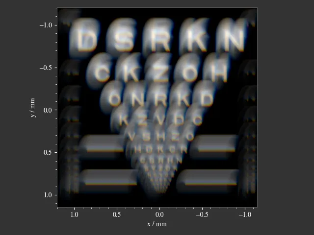
img = ot.presets.image.ETDRS_chart_inverted([0.5, 0.5])
psf = ot.presets.psf.halo()
convolve is then called in the following way:
img2 = ot.convolve(img, psf, m=0.5)
It returns the convolved image object img2.
When img and psf are of type GrayscaleImage, img2 is also a GrayscaleImage.
For all other cases color information are generated and img2 is a RGBImage.
Slicing and Padding
When doing a convolution, the output image size is extended by half the PSF size in each direction.
By providing keep_size=True the padded data can be neglected for the resulting image.
img2 = ot.convolve(img, psf, m=0.5, keep_size=True)
The convolution operation requires data outside the image. By default, the image is padded with zeros prior convolution.
Other modes are also available. For instance, padding with white color is done in the following fashion:
img2 = ot.convolve(img, psf, m=0.5, keep_size=True, padding_mode="constant", padding_value=1)
padding_value specifies the values used for constant padding for each channel.
Depending on type of the input img, it should be provided as either single value of a list of three values.
Typically, edge padding is a viable choice for reducing boundary effects:
img2 = ot.convolve(img, psf, m=0.5, keep_size=True, padding_mode="edge")
Color conversion
The colored image convolution can produce colors outside of the sRGB gamut.
To specify a defined color mapping, conversion arguments can be provided by the cargs argument.
By default they are set to dict(rendering_intent="Absolute", normalize=True, clip=True, L_th=0, chroma_scale=None).
Provide a cargs dictionary to override this setting.
img2 = ot.convolve(img, psf, m=0.5, keep_size=True, padding_mode="edge", cargs=dict(rendering_intent="Perceptual"))
The above command overrides the rendering_intent, while leaving the other default options unchanged.
Normalization
For a GrayscaleImage PSF, the PSF is automatically normalized inside the convolution function
so the overall power is one. By also setting cargs=dict(normalize=False), the output image won’t be
normalized, meaning brightness/color values are not rescaled automatically.
This is useful when the input image does not include any bright areas,
therefore does not use full available intensity range.
However, this is only supported for GrayscaleImage PSF.
4.11.5. Image Examples
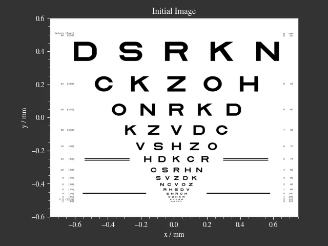
|
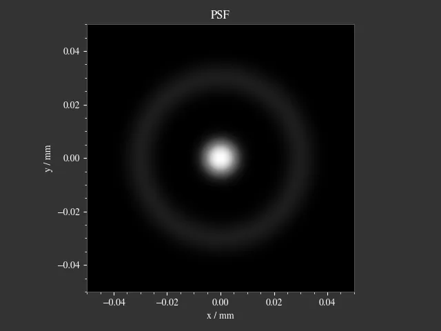
|
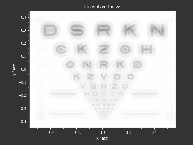
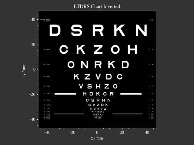
|
|
4.11.6. Presets
The are multiple PSF presets available.
All functions return a GrayscaleImage, with intensities linear to human perception.
For convolution, they are automatically converted to linear physical intensities inside the convolution function.
The functions below describe the mathematical formulations for the physical intensities.
Circle
A circular PSF is defined with the d circle parameter only:
psf = ot.presets.psf.circle(d=3.5)
Gaussian
A simple Gaussian intensity distribution is described as:
The shape parameter sig defines the Gaussian’s standard deviation:
psf = ot.presets.psf.gaussian(sig=2.0)
Airy
The Airy function is:
Where \(J_1\) is the Bessel function of the first kind of order 1.
The resolution limit r is described as distance from the center to the first root.
psf = ot.presets.psf.airy(r=2.0)
Glare
A glare is modelled as two different Gaussians, a broad and a narrow one Parameter \(a\) describes the relative intensity of the larger one.
psf = ot.presets.psf.glare(sig1=2.0, sig2=3.5, a=0.05)
Halo
A halo is modelled as a central Gaussian and annular Gaussian function around \(r\). \(\sigma_1, \sigma_2\) describe the standard deviations of both. \(a\) corresponds to the intensity of the ring.
psf = ot.presets.psf.halo(sig1=0.5, sig2=0.25, r=3.5, a=0.05)


