5.1. Property Sampling

5.1.1. Overview

Optrace approximates optical effects by utilizing an Unbiased Quasi Monte Carlo simulation. Inverse Transform Sampling is used as method for non-uniform random variate generation and Stratified Sampling as low discrepancy method for the generation of the initial uniform random variable.

A brief description of these terms:

Monte Carlo Simulation: An algorithm class that approximates a problem with many degrees of freedom by randomly choosing and simulating a subset of all property and variable combinations.

Quasi Monte Carlo Simulation: Monte Carlo Simulation, but the sampling is not truly random or pseudo-random. Instead it has some underlying deterministic or semi-deterministic nature to it. See low-discrepancy methods below.

Unbiased and Biased Methods: Performing an unbiased Monte Carlo simulation with an infinitely large set of samples produces an exact description of the physical system. Starting with few samples, with a larger and larger number the simulation converges towards the correct behavior. In contrast, a biased simulation never reaches a fully accurate description of the system. Biased methods can consist of neural network tasks or algorithms that comprise of some simplification of the system model. A more mathematical descriptions of biasedness can be found here: [1]

Non-Uniform Random Variate Generation: Generating random numbers, while some numbers are more likely to be chosen than others. The probability distribution is non-uniform.

Low Discrepancy Method: Methods that generate numbers, where the distribution of these values only deviates weakly from an equidistribution. White noise would be a high discrepancy method, since many samples are needed to approximate a true equidistribution. A regular value grid is a zero discrepancy method, since the values are always regularly distributed. Low discrepancy methods can be seen as a compromise between those two, trying to create values that fill an interval or area more uniformly than random values, but are less “obviously deterministic” than simple grids. Important types of low discrepancy methods include Hamilton and Sobol sequences as well as lattice methods.

Stratified Sampling: One of many low discrepancy methods. Random values are chosen from a set of sub-groups. It is guaranteed, that values are chosen from every sub-group (e.g. different intervals), but the values inside each sub-group are chosen randomly (e.g. random positions inside each interval). Details on the implementation in optrace are discussed in Section 5.1.5.

Inverse Transform Sampling: Generating non-uniform random numbers according to a known distribution function by utilizing the inverse transform method. Details on this method get discussed in Section 5.1.4. Important alternative sampling methods include: Importance Sampling, Rejection Sampling

5.1.2. Ray Properties

When generating rays at the source, there are multiple properties and property distribution. The number of degrees of freedom is dependent on the source parameters.

In the most simple case, with no degree of freedom, we have a monochromatic point source with parallel light and equal polarization. On the other end of the spectrum there is an area source with a broad spectrum, random polarization, an ray orientation dependent on the ray position and a randomly spreading rays relative to this orientation inside some directional cone.

Table 5.1 List of ray properties

Symbol	Description	Comment	Degrees of Freedom
\(x,y\)	Position	Point Source, Line Source, Area Source	0 - 2
\(\lambda\)	Wavelength	Monochromatic or spectrum	0 - 1
\(P\)	Power	All rays have equal power	0
\(s_0\)	orientation vector	Constant or position dependent	0 - 2
\(s\)	orientation vector distribution around \(s_0\)	Constant or specified as 1-2 angle distributions	0 - 2
\(E\)	Polarization	Constant or specified by angle distribution	0 - 1

For properties with one or two degrees of freedom the initial uniform random variable is created using stratified sampling in Section 5.1.5. So for instance for position sampling for an area the two dimensional stratified sampling creates the random variables \(\mathcal{U}_x,~\mathcal{U}_y\), which later gets used as input for position sampling in Section 5.1.9.

5.1.3. Stochastic Sampling

In raytracing, it is a standard procedure to randomize the beam properties. The advantage is that periodic artifacts and sampling errors are exchanged for noise. This approach is known as stochastic sampling [2].

An example is the sampling of a surface using a rectangular grid. With a violation of the sampling theorem aliasing occurs visible artifacts occur. The effect can be seen in [3], figure 4, and [4], slide 8.

However, if the rays are randomly distributed on the surface, the sampling theorem is still violated locally, but at random locations and randomly strong due to the random spacing between the sampling points. For the viewer, the resulting aliasing in the image appears as noise.

5.1.4. Inverse Transform Sampling

To calculate a random variable \(\mathcal{T}_{[0,1]}\) with probability distribution function \(\text{pdf}(x)\) from a uniform random variable \(\mathcal{U}_{[0,~1]}\) we make use of the inverse transform sampling theorem [5].

(5.1)\[\mathcal{T}_{[0,~1]} = \text{cdf}^{-1}\left(\mathcal{U}_{[0,~1]}\right)\]

Where \(\text{cdf}^{-1}(x)\) is the inverse cumulative distribution function. The cumulative distribution function \(\text{cdf}\) is defined as integral of a probability distribution function \(\text{pdf}\):

(5.2)\[\text{cdf}(x) = \int_{-\infty}^{x} \text{pdf}(\chi) ~\text{d}\chi\]

This can be generalized for sampling from an interval \([a,~b]\) of a function \(f(x)\) with

(5.3)\[F(x) = \int_{a}^{x} f(\chi)~\text{d}\chi\]

with \(F(x)\) being injective \(\forall x \in [a, b]\) as:

(5.4)\[\mathcal{T}_{[a,~b]} = \text{F}^{-1}\left(\mathcal{U}_{[\text{F}(a),~\text{F}(b)]}\right)\]

This fact is also explained in [5] under “Truncated Distributions” or in [6], last paragraph.

5.1.5. Stratified Sampling

Perrier[7] goes into great length to examine and compare different low-discrepancy methods in his work. Regarding simplicity, speed ([7], Figure 3.38), convergence ([7],Table 3.1), spectrum and discrepancy ([7], Figure 3.37) the stratified sampling method is most suitable in our raytracer. This method is described in [7], pages 36-37, while another explanation can be found in [8] under the name Uniform Sampling + Jitter.

One dimension

In one dimension the coordinate set \(\mathcal{X}_N\) with \(N\) values is made of an equally spaced interval values with an additional dither having the maximum size of one interval spacing.

(5.5)\[\mathcal{X}_N = \left\{\frac{i}{N} + \mathcal{U}_{[0,~1/N]} ~~:~~ i \in \mathbb{N}, ~0 \leq i < N\right\}\]

The set values then need to be randomly shuffled before using it.

Two dimensions

For simplicity, a square grid is used for stratified sampling in two dimensions. Each number can be divided into a square and remaining non-square part. The remaining part gets distributed randomly inside the grid.

\(N\) points can be divided into a root number \(N_s = \lfloor\sqrt{N}\rfloor\) and a remaining term \(\Delta N = N - N_s\). A set of rectangular grid coordinates with \(N_s\) values in each dimension is added with a dither to produce a stratified sampled grid \(\mathcal{P}_G\).

(5.6)\[\mathcal{P}_G = \left\{\left(\left\lfloor\frac{i}{N_s}\right\rfloor + \mathcal{U}_{[0,~1/N_s]}, ~i \;\text{mod}\; N_s + \mathcal{U}_{[0,~1/N_s]} \right) ~~:~~ i \in \mathbb{N}, ~0 \leq i < N_s^2\right\}\]

Remaining points \(\mathcal{P}_\Delta\) are generated randomly inside the grid, being equivalent to white noise sampling:

(5.7)\[\mathcal{P}_\Delta = \left\{\left(\mathcal{U}_{[0,~1]}, ~\mathcal{U}_{[0,~1]} \right) ~~:~~ i \in \mathbb{N}, ~0 \leq i < \Delta N\right\}\]

The point set \(\mathcal{P}\) with size \(N\) is then the union of both:

(5.8)\[\mathcal{P} = \mathcal{P}_G \cup \mathcal{P}_\Delta\]

The set \(\mathcal{P}\) then needs to be randomly ordered.

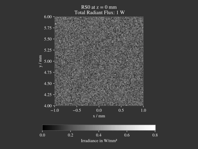
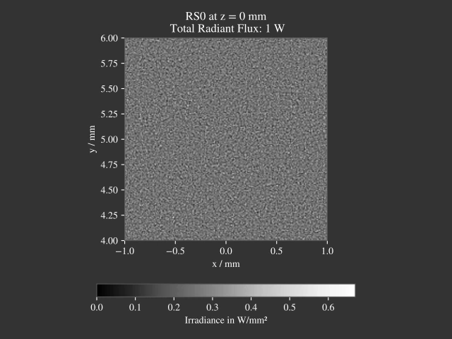
Comparison with simple sampling

A comparison to simple sampling (white noise generation) can be found in the following figures.

Fig. 5.1 200k rays on a square area with simple uniform sampling, image rendered with 189 x 189 pixel

Fig. 5.2 200k rays on a square area with two dimensional stratified sampling, image rendered with 189 x 189 pixel

5.1.6. Disc/Annulus Sampling

Polar Grid Transformation Artifacts

Stratified sampling generates a rectangular grid, which for a circular surface needs to be transformed into a polar grid. While this is done uniformly in Section 5.9.4, there are some circular artefacts visible, especially at the center.

Fig. 5.3 200k rays with stratified sampling and a polar grid transformation as done in Section 5.9.4, image rendered with 189 x 189 pixel

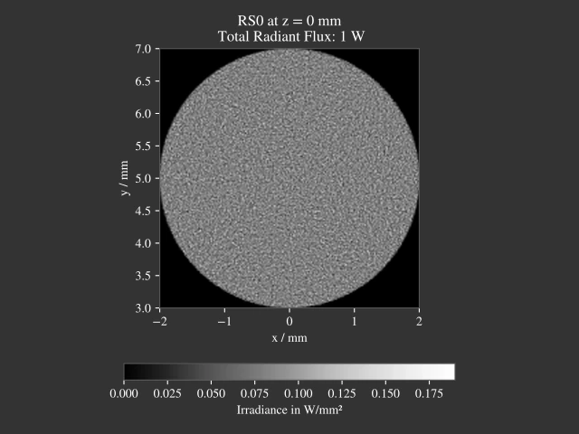
Fig. 5.4 200k rays on a circular area with positions mapped from stratified grid, image rendered with 189 x 189 pixel

These artifacts arise from the highly distorted initial rectangular cells, that in those regions become circular sectors. At the disc edge the rectangular cells are less distorted. In the inner region the area elements consist of small arc lengths and a large radial component, while going further outside the arc lengths increase and the radial lengths decrease. Near the center the area elements appear zoomed in. You can see such a grid and its distortion in [9], figure 5, as well as the alternative method that is showcased next.

Although for many rays the mentioned artefacts become less and less visible, a different approach should be desirable. This is especially important as the center of the disc typically lies at the optical axis or, when generating direction distributions, at the center direction of the distribution volume.

Square to Disc Mapping

One improved method is the Square-Disc Mapping method from [9]. optrace implements a simplified method from [10]. Sampled grid values \(x,~y\) lie inside a grid with bounds \(([-r_\text{o}, ~r_\text{o}], ~[-r_\text{o}, ~r_\text{o}])\) and get transformed to radial disc coordinates with:

(5.9)\[\begin{split}(r, \varphi)= \begin{cases}\left(x, ~\frac{\pi}{4} \frac{y}{x}\right) & \text { if } x^2>y^2 \\ \left(y, ~\frac{\pi}{2}-\frac{\pi}{4} \frac{x}{y}\right) & \text { if } x^2 \leq y^2 \text { and } y^2>0 \\ (0,~0) & \text { otherwise } \end{cases}\end{split}\]

Where \(r_\text{o}\) is the outer radius of the circle. Note that \(r\) has a sign, contrary to polar coordinates.

Disc to Annulus Mapping

When a annulus (surface between to concentric circles) is required, the disc coordinates can be transformed by rescaling the radius \(r\) non-linearly. In Section 5.9.4 we talk about how the linear values need to be inserted into a square function to achieve an equal-area mapping for a ring. The mapped radius \(r_\text{A}\) from an annulus with inner radius \(r_\text{i}\), outer radius \(r_\text{o}\) and radial coordinates \(r \in [0,~r_\text{o}]\) from (5.9) is then:

(5.10)\[\begin{split}r_\text{A} = \begin{cases} \text{sign}(r) \sqrt{r^2_\text{i} + r^2 \left(1 - \frac{r^2_\text{i}}{r^2_\text{o}}\right)} & \text{ if } r \neq 0\\ r_\text{i} & \text{ if } r = 0\\ \end{cases}\end{split}\]

5.1.7. Power Sampling

The same power value is assigned to all rays.

5.1.8. Polarization Sampling

For generating linear ray polarizations the procedure in Section 5.2.3 is applied. \(s = [0, 0, 1]\) is a vector parallel to the optical axis and \(s' \in \mathcal{S}\) from the directions generated above. The initial polarization \(E\) lies in the xy-plane and has some randomly distributed angle \(\mathcal{A}\) inside this plane.

(5.11)\[\begin{split}E = \begin{pmatrix} \cos \mathcal{A}\\ \sin \mathcal{A}\\ 0 \end{pmatrix}\end{split}\]

Following this procedure, we get \(E'\), which is the polarization vector at the source.

The advantage of simulating the polarization vector after a virtual lens can be demonstrated using the following example:

1. Generating ray vectors \(e_z = [0, 0, 1]\) with an polarization angle \(\alpha\). These rays get focused by an ideal lens, that has a well-defined focal point. Rays in this focal point have some vector distribution \(\mathcal{S}\) and a polarization distribution \(\mathcal{E}'\). The focal point can be seen as a point source.

2. Generating a point source with the same orientation vector distribution \(\mathcal{S}\) and polarization angle \(\alpha\) creates the same polarization distribution \(\mathcal{E}\)’ as in point 1. We can therefore omit this lens from before.

With this concept in mind, it now should be clear, what providing a fixed polarization angle or distribution means for different source ray directions.

The following angle distributions \(\mathcal{A}\) with \(\alpha \in \mathcal{A}\) are available:

Table 5.2 Polarization angle modes

x-Polarization	\(\alpha = 0^{\circ}\)
y-Polarization	\(\alpha = 90^{\circ}\)
Constant Angle	\(\alpha = \alpha_0\)
xy-Polarization	\(\alpha\) randomly chosen from \(\{0^{\circ},~90^{\circ}\}\)
Uniformly distributed	\(\mathcal{A} = \mathcal{U}_{[0, ~2\pi]}\)
User Function	function \(f(\alpha)\) \(\mathcal{A} = F^{-1}\left(\mathcal{U}_{[F(\alpha_0), ~F(\alpha_1)]}\right)\)
List	angles \(A=\left\{\alpha_0, ~\alpha_1,~\dots\right\}\) with probabilities \(P=\left\{p_0, ~p_1,~\dots\right\}\) \(\alpha\) gets then chosen randomly from \(A\) according to \(P\)

5.1.9. Position Sampling

If a source image is specified, the positions are chosen randomly according to the effective intensity distribution of the image, see Section 5.8.5.

When no image is specified, positions are chosen randomly inside the source area, whereas the ray position probability density is uniformly random.

A Point source requires no sampling. 1D stratified sampling is employed for a Line source. A Rectangle surface is sampled by the 2D stratified sampling. For arbitrary rectangle aspect ratios the square sample grid cells become rectangular. A Circle or Ring surface get sampled according to the Disc/Annulus sampling section.

5.1.9.1. Spectrum Sampling

For a ray source with a sRGB image wavelengths are generated according to Section 5.8.5. In all other cases the wavelengths are chosen randomly according to a specified spectrum.

A Monochromatic type spectrum requires no random sampling. Sampling for Lines is implemented by a random selection of all wavelengths with weights proportional to their power. For types Constant and Rectangle the stratified 1D sampling is applied. Inverse transform sampling is applied for types User Function/ User Data / Blackbody.

A Gaussian type spectrum is truncated to allow only wavelength inside the visible spectrum. \(\lambda\) is limited to \(\lambda \in [\lambda_l,~\lambda_r]\). For this function the anti-derivative integration bounds \(\xi_a,~\xi_b\) need to be calculated first before performing the inverse transform method.

(5.12)\[\begin{split}\xi_a =&~ \frac{1}{2}\left(1 + \text{erf}\left(\frac{\lambda_\text{l} - \lambda_0}{\sqrt{2} \sigma_\lambda}\right)\right)\\ \xi_b =&~ \frac{1}{2}\left(1 + \text{erf}\left(\frac{\lambda_\text{r} - \lambda_0}{\sqrt{2} \sigma_\lambda}\right)\right)\end{split}\]

Where \(\lambda_0\) is the center wavelength and \(\sigma_\lambda\) the standard deviation. With these bounds the random wavelengths are then:

(5.13)\[\Lambda = \lambda_0 + \sqrt{2} ~ \sigma_\lambda ~ \text{erf}^{-1}\left(2\,\mathcal{U}_{[\xi_a, ~\xi_b]}-1\right)\]

5.1.10. Direction Cone

Modelling diffuse light emission is implemented by distributing ray directions around a base orientation \(s_0\). Around this vector rays are distributed inside a cone with half opening angle \(\theta_\text{max}\) with \(0 \leq \theta_\text{max} < \frac{\pi}{2}\). A direction vector \(s\) may have some opening angle \(\theta\) with \(0 \leq \theta \leq \theta_\text{max}\) and an angle \(\alpha\) inside the \(s_x,~s_y\)-plane perpendicular to the base cone orientation \(s_0\). However, \(s_x,~s_y\) are not parallel to the cartesian \(x,y,z\) axes, but arise from a vector multiplication of the cartesian axis and the base vector.

Fig. 5.5 Exemplary direction vector \(s\) inside a cone volume around \(s_0\)

With \(x = [1, 0, 0]\) and \(s_0\) being the base orientation unity vector for the cone the vectors \(s_x,s_y\) are calculated using vector products:

(5.14)\[\begin{split}\begin{align} s_y =&~ \frac{x \times s_0}{||x \times s_0||}\\ s_x =&~ s_0 \times s_y \end{align}\end{split}\]

Ray direction \(s\) is composed of the base vector \(s_0\) and a perpendicular component \(s_r = s_x \cos \alpha + s_y \sin \alpha\). Keeping trigonometric relations in mind, the resulting vector is also an unity vector, like all the input vectors.

(5.15)\[s = s_0 \cos \theta + \left( s_x \cos \alpha + s_y \sin \alpha\right) \sin \theta\]

The corresponding random variables for \(\theta,~\alpha,~s\) are \(\Theta,~\mathcal{A},~\mathcal{S}\).

5.1.11. 2D Direction Sampling

Ray directions are distributed inside a plane, which is a cross section of the cone in Section 5.1.10 including \(s_0\). Let \(\mathcal{A}\) be the random variable for \(\alpha\) with sample space \(\Omega_\alpha = \{\alpha_0, ~\alpha_0 + \pi\}\) with equal probability for each value. While \(\mathcal{A}\) is equal for all elements, distribution \(\Theta\) differs according to the desired behavior:

Function

For a function \(f(\theta)\) with \(\theta \in [0, ~\theta_\text{max}]\) and \(0 < ~\theta_\text{max} \leq ~\frac{\pi}{2}\) we can apply the inverse sampling theorem (5.4):

(5.16)\[\Theta = \text{F}^{-1}\left(\mathcal{U}_{[\text{F}(0),~\text{F}(\theta_\text{max})]}\right)\]

Isotropic

Isotropic means nothing different than uniformly in all directions, which here just means:

(5.17)\[\Theta = \mathcal{U}_{[0, ~\theta_\text{max}]}\]

Lambertian

A Lambertian radiator follows the cosine law. With \(f(\theta) = \cos \theta\), \(F(\theta) = \sin \theta\) and \(F^{-1}(F) = \arcsin(F)\) inverse transform sampling can be performed:

(5.18)\[\Theta = \arcsin \left(\mathcal{U}_{[0,~\sin \theta_\text{max}]}\right)\]

5.1.12. 3D Direction sampling

For generating a direction cone two random variables are needed. To achieve an uniform, stratified and artefact free distribution, the disc mapping from Section 5.1.6 is applied. The random variable \(\mathcal{A}\) for values of \(\alpha\) is made of values of \(\theta\) from disc mapping. The second uniform variable \(\mathcal{U}\) is then the radius squared \(r^2\) and normalized by the squared disc radius.

(5.19)\[\mathcal{U}_{[0,~1]} = \frac{r^2}{r^2_\text{o}}\]

Squaring is necessary as the values are uniformly distributed according to the area, but we need uniformly distributed values according to the radius. The inverse transformation for this is known from Section 5.9.4. Rescaling this uniform variable into the desired output range is a simple linear transformation.

Function

Let \(f(\theta)\) be a user function with \(\theta \in [0, ~\theta_\text{max}]\) with \(0 < \theta_\text{max} \leq \frac{\pi}{2}\). In three dimensions \(f(\theta)\) needs to be scaled with \(\sin \theta\) for the distribution function, see [11] under Create samples on the hemisphere.

\(g(\theta)\) is then defined as \(g(\theta) := f(\theta) \sin \theta\). We can apply the inverse sampling theorem (5.4) on this new function:

(5.20)\[\Theta = \text{G}^{-1}\left(\mathcal{U}_{[\text{G}(0),~\text{G}(\theta_\text{max})]}\right)\]

Isotropic

With \(f(\theta) = 1\) we get \(g(\theta) = \sin \theta\) and \(G(\theta) = 1-\cos \theta\) and \(G^{-1}(G) = \arccos (1-G)\). Bounds are \(G \in [0, ~1-\cos \theta_\text{max}]\) and \(1 - G \in [1, ~\cos \theta_\text{max}]\). The latter get swapped to ensure ascending bounds.

(5.21)\[\Theta = \arccos\left(\mathcal{U}_{[\cos \theta_\text{max}, ~1]}\right)\]

This is consistent with [12].

Lambertian

For \(f(\theta) = \cos \theta\) we get \(g(\theta) = \cos \theta \sin \theta\) and \(G(\theta) = \frac{1}{2} \sin^2 \theta\). The anti-derivative inverse is then \(G^{-1}(G) = \arcsin \sqrt{2G}\) with bounds \(\{0, ~\frac{1}{2}\sin^2 \theta_\text{max}\}\). A uniform random variable \(2G\) is then bound to \(\{0, \sin^2 \theta_\text{max}\}\).

For the angle distributions we get a form that is consistent with [13]:

(5.22)\[\Theta = \arcsin\left(\sqrt{\mathcal{U}_{[0, ~\sin^2 \theta_\text{max}]}}\right)\]

---

References

[1]

Scratchapixel. Mathematical Foundations of Monte Carlo Methods. 2022. URL: https://www.scratchapixel.com/lessons/mathematics-physics-for-computer-graphics/monte-carlo-methods-mathematical-foundations/estimators.html (visited on 2022-12-01).

[2]

Robert L. Cook. Stochastic Sampling and Distributed Ray Tracing, pages 161–162. Acadenuc Press Limited, 1989.

[3]

Scratchapixel. Monte Carlo Methods in Practice. 2022. URL: https://www.scratchapixel.com/lessons/mathematics-physics-for-computer-graphics/monte-carlo-methods-in-practice/introduction-quasi-monte-carlo.html (visited on 2022-12-12).

[4]

Matthias Teschner. Advanced Computer Graphics - Sampling. 2015. URL: https://cg.informatik.uni-freiburg.de/course_notes/graphics2_04_sampling.pdf (visited on 2022-12-12).

[5] (1,2)

Wikipedia. Inverse transform sampling. 2022. URL: https://en.wikipedia.org/wiki/Inverse_transform_sampling (visited on 2022-12-01).

[6]

Rick Wicklin. The inverse cdf method for simulating from a distribution. 2013. URL: https://blogs.sas.com/content/iml/2013/07/22/the-inverse-cdf-method.html (visited on 2025-03-07).

[7] (1,2,3,4,5)

Helène Perrier. Anti-Aliased Low Discrepancy Samplers for Monte Carlo Estimators in Physically Based Rendering. Theses, Université de Lyon, March 2018. URL: https://theses.hal.science/tel-01801347.

[8]

Alan Wolfe. When Random Numbers Are Too Random: Low Discrepancy Sequences. 2017. URL: https://blog.demofox.org/2017/05/29/when-random-numbers-are-too-random-low-discrepancy-sequences/ (visited on 2022-12-01).

[9] (1,2)

Peter Shirley and Kenneth Chiu. A low distortion map between disk and square. Journal of Graphics Tools, 2(3):45–52, 1997. doi:10.1080/10867651.1997.10487479.

[10]

Pete Shirley. Improved code for concentric map. 2011. URL: https://psgraphics.blogspot.com/2011/01/improved-code-for-concentric-map.html (visited on 2022-12-17).

[11]

Scratchapixel. Global Illumination and Path Tracing. 2022. URL: https://www.scratchapixel.com/lessons/3d-basic-rendering/global-illumination-path-tracing/global-illumination-path-tracing-practical-implementation.html (visited on 2022-12-06).

[12]

Wolfram MathWorld. Sphere Point Picking. 2022. URL: https://mathworld.wolfram.com/SpherePointPicking.html (visited on 2022-12-06).

[13]

Particle In Cell Consulting LLC. Modeling Diffuse Reflection (or How to Sample Cosine Distribution). 2015. URL: https://www.particleincell.com/2015/cosine-distribution/ (visited on 2022-12-06).